18 Control systems
The book is still taking shape, and your feedback is an important part of the process. Suggestions of all kinds are welcome—whether it’s fixing small errors, raising bigger questions, or offering new perspectives. I’ll do my best to respond, but please keep in mind that the text will continue to change significantly over the next two years.
You can share comments through GitHub Issues.
Feel free to open a new issue or join an existing discussion. To make feedback easier to address, please point to the section you have in mind—by section number or a short snippet of text. Adding a label characterizing your issue would also be helpful.
Last updated: November 15, 2025
18.1 Control systems overview
Images are captured under a wide variety of conditions, and there is no single set of parameters—such as focus, exposure time, or sensor gain—that guarantees high-quality results in every situation. To address this, sensors are equipped with control systems that automatically adjust acquisition parameters. These systems help prevent pixel saturation, reduce image noise, and set optical properties like focal plane and depth of field. In computer vision applications, such as robotics or autonomous driving, these control systems are essential for obtaining reliable quantitative data. In consumer photography, they assist users in quickly achieving settings that produce visually appealing images.
The sensor control systems are typically implemented by the commercial vendors. The general principles of these control methods can be described, but the specific implementations can be quite complex, with many parameters, and are trade secrets. Moreover, the control systems themselves need to be adjusted in various ways that depend on the details of the optics and sensor in the camera. This section describes the principles of the control systems. It is my view that there are opportunities to develop better open standards for designing and evaluating these control systems through simulation.
18.2 Focus Control
In some imaging applications, the lens position can be fixed. For example, consider an autonomous driving system where the camera is designed to detect vehicles or pedestrians at distances greater than 3 meters. With a focal length of 30 mm, the ideal sensor-to-lens distance for objects beyond 3 meters varies only slightly—from \(\frac{300}{299} \times 25\) mm to 25 mm—about \(83 \mu \text{m}\). Over this range, image sharpness remains nearly constant, with the effect depending mainly on the aperture size (see Section 9.15). In such cases, the lens can be set to focus at infinity, and no adjustment is needed.
However, in many other imaging systems, the camera must adjust the lens position to bring objects at different distances into focus. This is especially important in consumer photography, for close-up portraits or enabling the photography to put some objects into focus while blurring the background.
18.2.1 Lens Positioning in SLR and DSLR Cameras
In single-lens reflex (SLR) and digital SLR (DSLR) focus is usually achieved mechanically. The imaging lens -typically comprising multiple lenses and called either multi-element optics or a lens assembly- is mounted on a screw thread. The lens position is adjusted by rotating the assembly along the thread. The lenses are typically rotationally symmetric, so the rotation is irrelevant to the image quality. The thread pitch of the screw determines how finely the position can be adjusted.
SLR camera bodies and lenses are relatively large. I lugged quite a few of them around on trips. For my wife. Moving the entire assembly back and forth, called the unit focusing, is challenging. To lighten the load, lens designers created systems that could change the focus by moving only a small, relatively light, subgroup of lenses within the assembly. If the lenses were in the middle of the assembly, this was called internal focusing, and if the lenses were at the rear this was called rear focusing. Moving a small, internal group of lens elements is a sophisticated design that is fundamental to the performance of modern autofocus lenses and has several advantages.
- Faster and Quieter Autofocus: Moving a smaller, lighter group of elements requires a much smaller, less powerful motor. This allows for significantly faster, quieter, and more energy-efficient autofocus performance, which is critical for tracking moving subjects.
- Constant Lens Length: Because all the movement happens inside the sealed barrel, the overall physical length of the lens does not change during focusing. This improves the balance and handling of the camera and lens combination.
- Non-Rotating Front Element: The front of the lens does not move or rotate. This is a huge advantage when using filters like polarizers or graduated neutral density filters, which must be kept in a specific orientation to work correctly.
- Improved Optical Performance: By freeing designers from the constraint of moving the entire optical block, internal focusing allows for more complex and better-corrected optical formulas. It can lead to sharper images and better close-focusing capabilities.
SLR cameras represented a major advance over earlier rangefinder designs, and when I was young they were considered super cool. In a rangefinder camera, there are two separate optical paths:
- Imaging Lens: The main lens focuses the image onto the film or sensor, but you do not look through this lens.
- Viewfinder Window: A separate window on the camera body that you use to compose the shot.
Because the viewfinder and imaging lens are separate, the viewfinder image can differ slightly from what is captured on film or sensor, making precise framing more challenging.
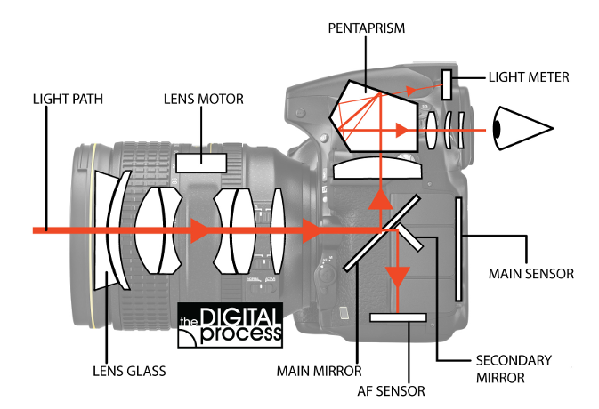
The innovation of the SLR (Single-Lens Reflex) camera is that it uses a single optical path for composing, focusing, and capturing the image—hence “single lens.” Light entering through the lens assembly is directed by a semi-transparent “reflex” mirror (a type of beam splitter). Typically, about 70% of the light is sent to the viewfinder, while the remainder is directed to the autofocus subsystem. When the shutter is pressed, the mirror flips out of the way, allowing all the light to reach the film (SLR) or digital sensor (DSLR) (Figure 18.1).
The SLR design also allows the user to control the aperture size, which directly affects the depth of field (Section 9.15). One advantage of this design is that you can preview changes in depth of field directly through the viewfinder.
18.2.2 Lens Positioning in Mobile Devices
DSLRs had a large volume compared to smartphones and other compact devices. These cameras also use much smaller multi-element lenses. Focus is commonly controlled by a voice coil motor (VCM), which is reliable, inexpensive, and widely used in the industry (Figure 18.2). The small motor moves the entire lens assembly.
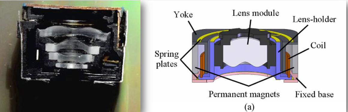
There is also a growing market for lens positioning in cell pones using Micro-Electro-Mechanical Systems (MEMS) devices. These devices offer advantages such as low power consumption, fast response, and miniaturization, making them attractive for mobile imaging systems. The difference, however, is not huge.
Conceptually, autofocus methods share similarities with techniques for estimating object distance. Both rely on understanding the optical light field (Section 2.6). While the implementation of autofocus algorithms has evolved significantly in recent years, the underlying physical principles remain the same. We begin with the classic autofocus mechanism and then describe more recent implementations that are integrated directly into CMOS sensors.
18.2.3 Phase Detection Autofocus (PDAF)
Figure 18.4 illustrates the principle of phase detection autofocus (PDAF). In this system, rays from a point object near the lens travel through different parts of the aperture—red rays from the top and green rays from the bottom—before reaching the sensor. When the lens is correctly focused, these rays converge to a single point on the sensor, producing a sharp image.
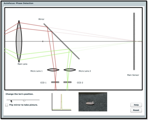
The classic PDAF design, invented in the 1970s, uses a partially reflective mirror behind the main lens to direct light from the top and bottom of the lens to two separate microlenses. Each microlens focuses the incoming rays onto a linear sensor array. The system is arranged so that, when the image is in focus, the light from both the top and bottom of the lens is centered on their respective arrays. If the image is out of focus, the rays are displaced from the centers of the arrays. The relative displacement—called the phase difference—indicates both the amount and direction of defocus.
The autofocus subsystem uses this phase difference to determine how to move the lens to achieve focus. This method became a key feature in single-lens reflex (SLR) cameras, enabling fast and accurate autofocus.
However, this approach has drawbacks. The mirror, microlenses, and sensor arrays require a relatively large and complex mechanical assembly, making it impractical for compact devices like smartphones. Additionally, the system can only perform focusing or image capture at one time, not both simultaneously. Later technologies addressed these limitations.
Phase detection autofocus (PDAF) for SLR cameras was pioneered by Honeywell, which patented the key concepts in the 1970s (U.S. Patents 3,875,401 and 4,185,191). Their design used a beam-splitting rangefinder rather than the later flip-mirror approach.
The first commercial SLR to feature PDAF was the Minolta Maxxum 7000 (α-7000 in Japan), released in 1985. It integrated in-body PDAF and motorized lens control, using phase differences measured by two linear sensor arrays to drive lens adjustments.
Leica had previously patented a different autofocus method based on contrast detection, which they licensed to Minolta. However, Minolta found this approach too slow and unreliable, so they developed a phase detection system instead—without securing a license from Honeywell. Honeywell sued and ultimately won a substantial award.
18.2.4 Dual Pixel Autofocus (DPAF)
Traditional phase detection autofocus (PDAF) systems are difficult to implement in the compact form factor of smartphones. As a result, manufacturers initially adopted methods called contrast detection autofocus (CDAF). These methods adjust the lens position to maximize image contrast, under the assumption that a well-focused image will have the sharpest edges. The CDAF methods lack a direct, physical measurement to guide lens movement, making it relatively slow and unreliable, especially in low-light or noisy conditions. Other approaches, such as time-of-flight (ToF) sensors (Section 20.9), have also been explored and are still used in some devices.
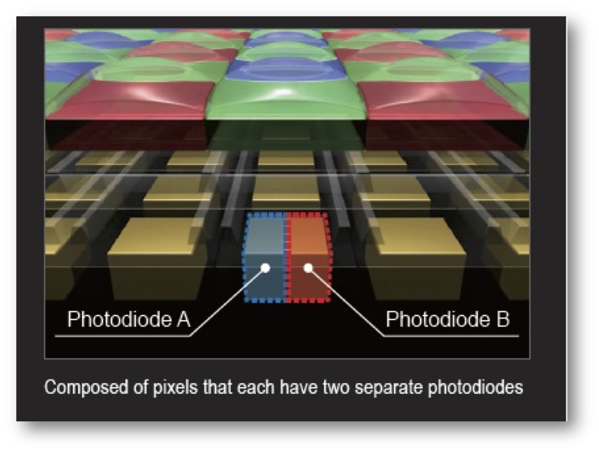
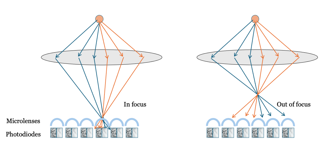
A major breakthrough came in 2014 with the introduction of dual pixel autofocus (DPAF), which applies the principles of phase detection directly within the CMOS sensor. In DPAF, each pixel (or a subset of pixels) contains two photodiodes beneath a single microlens (Figure 18.5). During normal image capture, the signals from both photodiodes are combined. For autofocus, however, the signals are read separately and compared.
Canon introduced DPAF with the EOS 70D in 2013, building on earlier hybrid PDAF/live-view systems like the EOS 650D/T4i-D. Today, many vendors—including Sony and Omnivision—ship sensors with two photodiodes under each microlens, enabling fast, accurate on-sensor phase detection autofocus, especially for video.
The underlying principle is based on the optical light field. For pixels near the center of the sensor, light rays from the left and right sides of the lens arrive at slightly different angles. The microlens directs these rays onto separate photodiodes within the pixel—one on the left, one on the right. When the image is in focus, both photodiodes receive similar signals. If the image is out of focus, the rays from the left and right sides of the lens are displaced, causing the signals from the two photodiodes to differ and shift relative to each other. The amount and direction of this shift indicate the degree and direction of defocus, just as in traditional PDAF.
By using two photodiodes under each microlens, DPAF sensors capture some information about the optical light field—the left and right subpixels sample rays from different parts of the lens. This concept could be extended further: with more subpixels, it may be possible to recover even richer light field information, opening up new possibilities for computational imaging and post-capture refocusing (Section 20.3).
18.3 Exposure Control
To capture a high-quality image, the exposure must be set so that dark regions generate enough electrons to rise above the sensor’s noise floor, while bright regions do not exceed the pixel’s full well capacity (Section 16.3). If the exposure time is too short, pixels in dark areas collect very few electrons—sometimes fewer than the noise level. Even with a low-noise sensor, the inherent Poisson noise means that a small number of electrons results in a low signal-to-noise ratio. For example, if a pixel collects an average of 4 electrons, the standard deviation is 2, so the SNR is only 2.
Conversely, if the exposure time is too long, pixels in bright areas may generate more electrons than the pixel can store, causing the floating diffusion node to saturate. When this happens, a wide range of scene intensities are all recorded at the same maximum value.
Proper exposure control adjusts acquisition parameters so that the scene’s dynamic range fits within the sensor’s dynamic range, avoiding both excessive noise and saturation. In a conventional system, two main parameters control this fit: the lens aperture size and the exposure duration. Increasing the aperture allows more light to reach the sensor, raising the signal level. Extending the exposure duration gives the sensor more time to collect photons and convert them to electrons. The classic specification for exposure combines these two parameters, as described below.
18.3.1 Exposure value
The exposure value (EV) is a single number that summarizes the combined effect of aperture size and exposure time on image brightness. For a lens with f-number \(F\) and exposure time \(T\) (in seconds), the exposure value is defined as
\[ \text{EV} = \log_{2}\left(\frac{F^2}{T}\right) = 2 \log_{2}(F) - \log_{2}(T) \tag{18.1}\]
A lower EV means either a longer exposure time or a wider aperture (smaller \(F\)), both of which allow more light to reach the sensor. As scene brightness increases, a higher EV is needed to avoid overexposure. For example, if \(F = 1\) and \(T = 1\) second, then \(EV = 0\). If the image is too bright and pixels are saturated, you can either halve the exposure time to \(T = 1/2\) second (raising \(EV\) to 1), or keep \(T = 1\) second and increase the f-number to \(F = \sqrt{2}\) (also \(EV = 1\)). Both changes reduce the light reaching the sensor by half1.
In film cameras, where each exposure was costly, photographers often used a separate light meter to determine the correct aperture and exposure time. Modern electronic cameras estimate scene brightness automatically, usually by taking continuous measurements just before the main exposure. On DSLRs, this process is typically triggered by pressing the shutter button halfway. In smartphones, exposure estimation usually begins as soon as the camera app is opened.
18.3.2 Exposure Bracketing
A common engineering strategy for finding optimal settings is to perform a parameter sweep—systematically varying a parameter to observe its effect. In imaging, this is known as exposure bracketing.
Exposure bracketing means capturing several images of the same scene at different exposure durations. The technique dates back to at least 1851, when Gustave Le Gray photographed seascapes by taking separate exposures for the sky and the sea, since film could not capture both correctly in a single shot.
Modern digital cameras often provide an exposure bracketing feature. Typically, the user selects the best image from the set, but it is also possible to combine the bracketed images to create a composite with improved dynamic range.
18.3.3 Burst Photography
To prevent pixel saturation, a team at Google proposed capturing a sequence of images using short exposure durations—a technique known as burst photography Hasinoff et al. (2016). Their method involves aligning the individual images and summing them to reduce shot noise (Section 14.6).
This approach is particularly effective when sensor read noise is low and shot noise is the dominant noise source. In this scenario, each pixel measurement can be modeled as a Poisson random variable with mean \(\lambda\). Summing \(N\) such measurements yields another Poisson variable with mean \(N\lambda\), improving the signal-to-noise ratio.
The main advantage of burst photography is that it allows the use of short exposures to avoid saturation in bright regions, while still achieving high image quality by combining multiple frames. However, this method requires accurate alignment of the images. If there is motion in the scene or camera shake—especially if objects move in front of one another (occlusion)—alignment becomes challenging or may fail. Burst photography works best with static scenes and a stable camera, but can still provide benefits in more dynamic situations, even if not every frame can be perfectly aligned.
18.3.4 Space-varying exposure duration
The entire problem of exposure control becomes greatly simplified if there is not one exposure time, but there is a space-varying exposure time. In that case, the pixels in dark parts of the image can have a longer exposure time than pixels in the light part. This idea was implemented by the digital pixel sensor (Section 15.11). Recall that the voltage on each pixel, or small group of pixels, was measured non-destructively by the ADC. The voltage (\(v_i\)) and sample time (\(t_i\)) were recorded for the \(i^{th}\) pixel. These two values, together, estimate the effective intensity (\(E = v_i / t_i\)).
Using only the last non-saturated read in a DPS provides a higher SNR than combining exponentially spaced earlier reads — particularly when the number of reads is small and the sensor is near saturation.
In digital pixel sensors (DPS), it is common to sample the photodiode voltage multiple times during exposure. These samples can be taken at exponentially spaced time points to extend dynamic range. Suppose the sample times are given by
\[ t_i = t_0 \cdot 2^{i-1}, \quad \text{for } i = 1, 2, \dots, k, \]
with corresponding measurements
\[ V_i = \alpha t_i + n_i, \]
where \(\alpha\) is the photon flux (in electrons per unit time), and \(n_i \sim \mathcal{N}(0, \sigma_r^2)\) is independent Gaussian read noise.
We consider two estimators for \(\alpha\):
18.3.5 Using the Last Valid Read
If we estimate the flux using only the last read before saturation:
\[ \hat{\alpha}_{\text{last}} = \frac{V_k}{t_k}, \]
then the signal-to-noise ratio (SNR) is
\[ \mathrm{SNR}_{\text{last}} = \frac{\alpha t_k}{\sigma_r}. \]
18.3.6 Using Linear Regression
Using all \(k\) samples in a least-squares fit to estimate \(\alpha\), the variance of the slope estimator is
\[ \mathrm{Var}(\hat{\alpha}_{\text{reg}}) = \frac{\sigma_r^2}{\sum_{i=1}^k (t_i - \bar{t})^2}, \]
with
\[ \bar{t} = \frac{1}{k} \sum_{i=1}^k t_i = \frac{t_0 (2^k - 1)}{k}. \]
The sum of squared deviations becomes
\[ \sum_{i=1}^k (t_i - \bar{t})^2 = \sum_{i=1}^k t_i^2 - k \bar{t}^2 = t_0^2 \left( \frac{4^k - 1}{3} - \frac{(2^k - 1)^2}{k} \right). \]
Thus, the regression SNR is
\[ \mathrm{SNR}_{\text{reg}} = \frac{\alpha \sqrt{ \sum (t_i - \bar{t})^2 }}{\sigma_r}. \]
We compare the two:
\[ \frac{\mathrm{SNR}_{\text{reg}}}{\mathrm{SNR}_{\text{last}}} = \frac{ \sqrt{ \sum (t_i - \bar{t})^2 } }{ t_k } = \frac{1}{2^{k-1}} \sqrt{ \frac{4^k - 1}{3} - \frac{(2^k - 1)^2}{k} }. \]
18.3.7 Numerical Examples
| \(k\) | \(\mathrm{SNR}_{\text{reg}} / \mathrm{SNR}_{\text{last}}\) |
|---|---|
| 2 | 0.35 |
| 3 | 0.54 |
| 4 | 0.67 |
| 5 | 0.75 |
As the table shows, the regression estimator has lower SNR (ratio less than 1) than the last sample for small \(k\). Early reads contain less signal but still contribute read noise, diminishing the benefit of regression.
The f-number is the ratio of the focal length to the aperture diameter (Section 9.12). For a fixed focal length, increasing the f-number means reducing the aperture diameter, so less light reaches the sensor.↩︎