9 Thin lenses
The book is still taking shape, and your feedback is an important part of the process. Suggestions of all kinds are welcome—whether it’s fixing small errors, raising bigger questions, or offering new perspectives. I’ll do my best to respond, but please keep in mind that the text will continue to change significantly over the next two years.
You can share comments through GitHub Issues.
Feel free to open a new issue or join an existing discussion. To make feedback easier to address, please point to the section you have in mind—by section number or a short snippet of text. Adding a label characterizing your issue would also be helpful.
Last updated: October 15, 2025
9.1 Thin lenses overview
Many image system properties can be summarized by the geometric optics of ray tracing. This analysis characterizes important performance characteristics of an optical system, such as its focal length, magnification, and depth of field. These optical properties can be analyzed in a particularly simple and clear way if we consider very simple thin lenses.
Starting with an analysis of a thin lens has much practical value. First, many people, including both engineers and photographers, rely on the thin lens ideas when they describe optical system characteristics. Familiarity with these ray trace characterizations is important for anyone working in the field of image systems engineering. Second, even more complex image systems are often made from lenses that are well approximated by a collection thin lenses. We will go on to see how to extend the thin lens ideas to more complex systems in Chapter 10.
This section explains ways to understand image system optics by ray tracing. Important as it is, ray tracing is not up to the task of a full image systems simulation. As we saw in Chapter 7, we will need to account for the wave properties of light, for example to incorporate diffraction. We will explain the methods used for simulating the spectral irradiance at the sensor in subsequent chapters about linear systems (Chapter 11) and wavefront calculations (Chapter 13).
9.2 Lens diagram coordinates
To begin, let’s establish the conventional coordinates for illustrations of lenses and rays. Typically, light rays arerepresented as traveling from left to right and the direction of light ray travel is labeled as the \(z\)-axis. The object side, where the rays start, has negative \(z\) values and the image side has positive \(z\) values. The vertical direction in these diagrams is labeled the \(y\)-axis.
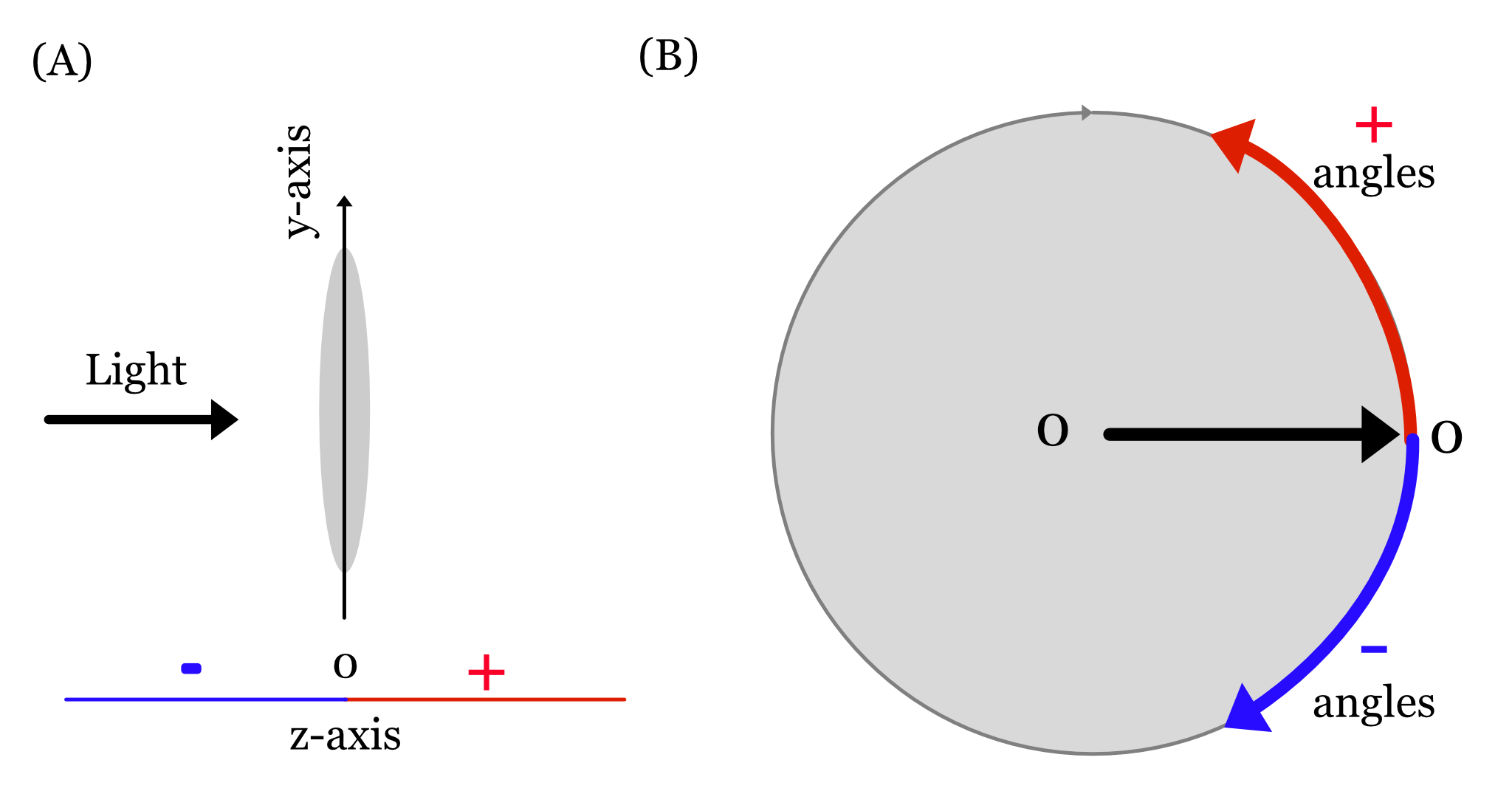
The ray angle is measured with respect to the \(z\)-axis, which is also called the optical axis. The counter-clockwise direction is a positive angle. I will use these coordinate throughout the book, unless for some reason I have to explicitly over-ride them. I hope that never happens.
9.3 What is a thin lens?
A lens is considered a thin lens when its axial thickness is negligible compared to the radii of curvature of its surfaces. The radius of curvature is the radius of a sphere whose surface matches the curvature of the lens surface. A lens with two convex surfaces (biconvex) will have two such radii, one for each of its surfaces.
While there isn’t a strict numerical rule, a common guideline is that the thin lens approximation is valid when the lens thickness is much smaller than its focal length and the radii of curvature of its surfaces. This approximation simplifies many optical calculations significantly.
Consistent with general lens coordinates (Figure 9.1), the radius of curvature is positive if its center of curvature is on the side of the outgoing light (typically to the right). It is negative if the center of curvature is on the side of the incoming light (typically to the left). In Figure 9.2, the left surface of the biconvex lens has a positive radius of curvature, while the right surface has a negative radius of curvature.
9.4 Focal points
Figure 9.3 shows the important concept of the primary and secondary focal points of a convex and concave thin lens. The primary focal point (F) is the location on the optical axis such that any ray coming from it towards the lens travels parallel to the axis after refraction. The distance from that point to the middle of the lens is called the focal length. The secondary focal point (F’) is the axial point such that any incident ray traveling parallel to the axis will, after refraction, proceed toward, or appear to come from it. The secondary focal point has its own focal length.
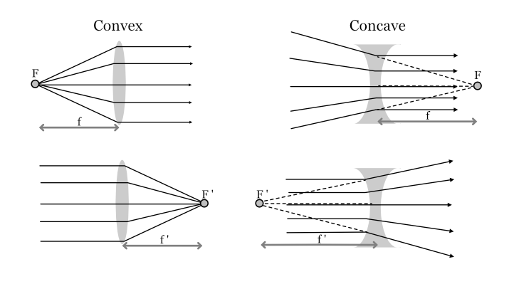
When examining the behavior of an equiconvex lens, two primary scenarios emerge. In the first scenario, rays emanating from the primary focal point (F) enter the lens and are refracted in such a way that they exit traveling parallel to the main optical axis. Conversely, when parallel rays enter the lens, they are refracted and converge towards the secondary focal point (F’), demonstrating the lens’s ability to redirect light.
The equiconcave lens presents a contrasting optical behavior. When incident rays enter the lens at various angles with the intention of producing parallel rays, these rays converge at the primary focal point (F) on the opposite side of the lens. Dashed lines can be used to trace and illustrate this convergence. In a separate scenario, when parallel rays enter the equiconcave lens, they diverge after refraction. If these diverging rays are extended backward using dashed lines, they appear to originate from the secondary focal point (F’) on the opposite side of the lens.
There are many useful calculations that one can explore with simple lenses and ray tracing. Here, we cover the basics to give the reader some of the terminology and a sense of how these systems are analyzed. For a deeper dive, I suggest the reader look into some of the excellent textbooks on optics (References here. Usually Goodman; Born and Wolf; I like Jenkins and White.)
9.5 Three ray tracing principles
Consider the vector object on the left of Figure 9.4. A ray from the arrowhead that is parallel to the axis will be refracted through the focal point. A ray from origin of the vector, which is on the optical axis, will also pass through the focal point. Finally, a ray from the arrowhead - and this is new - that passes through the center of the lens will continue on a straight path.
In summary, rays that
- Enter parallel to the optical axis and pass through the focal point on the opposite side.
- Pass through the center of the lens do not deviate (refract).
- Pass through the primary focal point toward the lens exit parallel to the optical axis.
9.6 Image plane
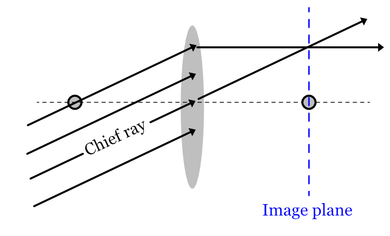
The rays from a distant point off the optical approach the entrance as parallel to one another but oblique to the optical axis. The ray that passes through the center of the lens is called the chief ray. There will also be a ray that passes through the primary focal point. It will be refracted by the lens and emerge as parallel to the optical axis. These two rays intersect where the image of the point will be formed.
9.7 Lens power (diopters)
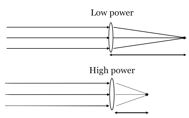
The power of a lens is the inverse of the focal length, in meters. The unit for lens power, \(1/m\) is the diopter. A short focal length implies large power, either due to the curvature of the lens surface or the refractive index of the lens material.
To measure the focal length of a lens we use a light source that produces parallel rays at the entrance aperture of the lens. We then slide the image plane back and forth, searching for the distance where the spot is smallest. We can create parallel rays using many methods. Perhaps the simplest is to use a small point source (e.g., an LED) at a distance from the lens. The rays arriving at the lens will be a small angular sliver of the emitted rays, and if the source is far from the lens the rays will be very close to parallel (e.g., Figure 7.3). An alternative, is to go outside on a sunny day and use the sun as a source. The sun isn’t small, but it is really far away. By the time the rays from the disk of the sun arrive at your lens, the rays will be parallel.
The optics in the human eye has multiple elements. Even so, we can measure its focal length, which is about 0.016 m (~60 diopters). To bring objects at different distances into focus the optics adjusts its power, a process called accommodation. If it cannot adjust adequately, we wear lenses (glasses, contact lenses) that increase or decrease the optical power, say by 1-8 diopters, so that a good image can be focused on the retina.
Young people can accommodate easily. As people age, we lose the ability to change the optical power of the optics, a condition called presbyopia. This happens to everyone. This biological fact is a consideration for the design of near field displays (Section 25.1).
9.8 The lens formula
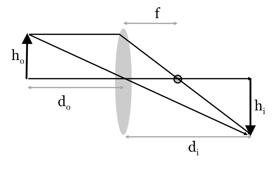
When an object is far away, the rays arriving at the lens are parallel. The image of the object will be in focus at the focal length. When the object is closer, we can use the Lens formula to find the plane where the object will be in focus. This is called the image distance. The equation, which was derived by Halley in 1693, relies on the three ray tracing properties of symmetric thin lenses (Section 9.5). Using these principles, we can locate where the object at a distance \(d_o\) will be in focused on the image side; call that distance \(d_i\).
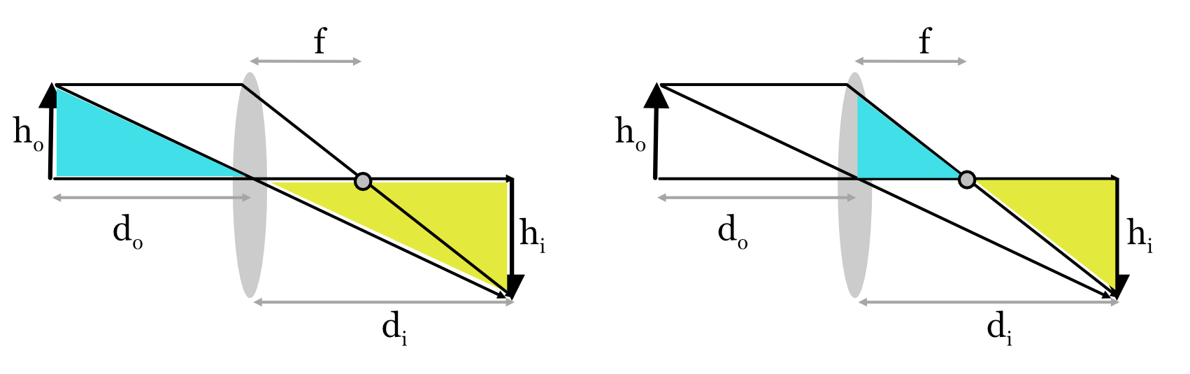
The rays in Figure 9.7 identify two pairs of similar triangles (cyan and yellow). On the left, we can see that the triangles imply \(h_i/h_o = d_i/d_o\). On the right, we can see that the triangle similarity implies \(h_i/h_o = \frac{d_i - f}{f}\). Combining the two equalities, we have
\[\frac{d_i}{d_o} = \frac{d_i - f}{f} = \frac{d_i}{f} - 1 \]
rearranging terms, \[ \frac{d_i}{f} = 1 + \frac{d_i}{d_o} \]
and dividing by \(d_i\) we have the lens formula
\[ \frac{1}{f} = \frac{1}{d_i} + \frac{1}{d_o} \tag{9.1}\]
The common names for these variables are
- \(d_o\) - Object distance
- \(d_i\) - Image distance
- \(f\) - Lens focal length
9.9 Image distance formula
Equation 9.1 defines a relationship between the object distance and the image distance for a thin lens. We can rearrange the terms.
\[ \frac{-1}{d_i} = \frac{1}{d_o} - \frac{1}{f} \]
Notice that when \(d_o = \infty\), then \(d_i = f\). We can re-write the formula to calculate the image distance explicitly.
\[ d_i = \frac{1}{\frac{1}{f} - \frac{1}{d_o}} = \frac{f~d_o}{d_o - f} \tag{9.2}\]
You can see from Equation 9.3 that as \(d_o\) becomes much larger than \(f\), \(d_i\) becomes approximately \(f\). Specifically, if we express \(d_o\) in terms of the focal length of the lens, \(k f\), we have
\[ d_i = \frac{f k f}{(k-1) f} = f \frac{k}{k-1} \tag{9.3}\]
This script plots the image distance as a function of object distance expressed as a multiple of focal length.
9.10 Lensmaker equation
The lens formula (Equation 9.3) relates the image distance, object distance, and focal length. The lens maker equation explains how to calculate the focal length of a thin lens. The formula applies to a thin lens with two spherical sides embedded in a homogeneous environment. To apply the formula, we must know the radius of curvature of the two sides of the lens as well as the index of refraction of the lens material and its surrounding medium.
Here is the formula:
\[ \frac{1}{f} = (\frac{n_2}{n_1} - 1) ( \frac{1}{R_1} - \frac{1}{R_2}) \tag{9.4}\]
Where - \(n_2\) is the refractive index of the lens - \(n_1\) is the refractive index of the surrounding medium - \(R_1\), \(R_2\) are the radii of curvature of the two surfaces
Here is a link to a very nice Khan Academy video derivation of the formula.
9.11 Biconvex lenses
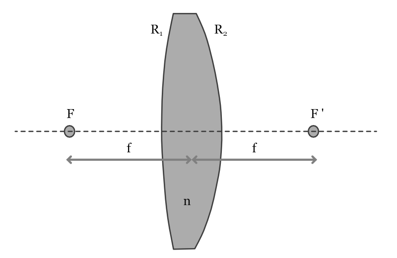
The lenses drawn in Figure 9.3 are symmetric (i.e., equiconvex and equiconcave), so it is not surprising, therefore, that the focal lengths of the primary and secondary focal points are equal. It is more surprising to learn that even if a thin lens has a different curvature on the two sides, the two focal lengths will still be equal Figure 9.8. Such lenses are called biconvex.
The symmetry follows from the formula in Equation 9.4. Exchanging the two radii of curvature simply changes the sign of the focal length.
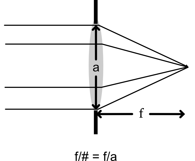
9.12 The \(\mathrm{f}/\#\) (f-number)
The \(~\mathrm{f}/\#\) of a thin lens is the ratio of its focal length and entrance aperture diameter (Figure 9.9). For example, when we write f/4, it means that the focal length is 4x the aperture diameter.
The \(~\mathrm{f}/\#\) is an important parameter for all thin lenses; this ratio appears in many formulae describing lens performance. It is the key parameter that defines many properties of a circular, diffraction-limited thin lens. Studying diffraction-limited lenses is an important case for evaluating image system performance because it represents an upper bound on the optical component; we cannot improve the image system performance by using better optics.
As an example, remember the formula for the Airy disk diameter (meters) on the image plane of a diffraction limited lens (Equation 7.1) in Section 7.3. That equation depends on the wavelength of light and the ratio of the focal length and aperture, which is the \(\mathrm{f}/\#\). Re-writing that formula, for a wavelength of \(\lambda\) and an \(~\mathrm{f}/\#\), we have
\[ d = 2.44 ~ \lambda ~ N \tag{9.5}\]
9.13 Magnification and zoom
Consider the simple thin lens in Figure 9.10 with a image distance of \(f = 0.1m\). We draw the rays to the image plane for an object at a distance of \(d_o = 0.3m\).
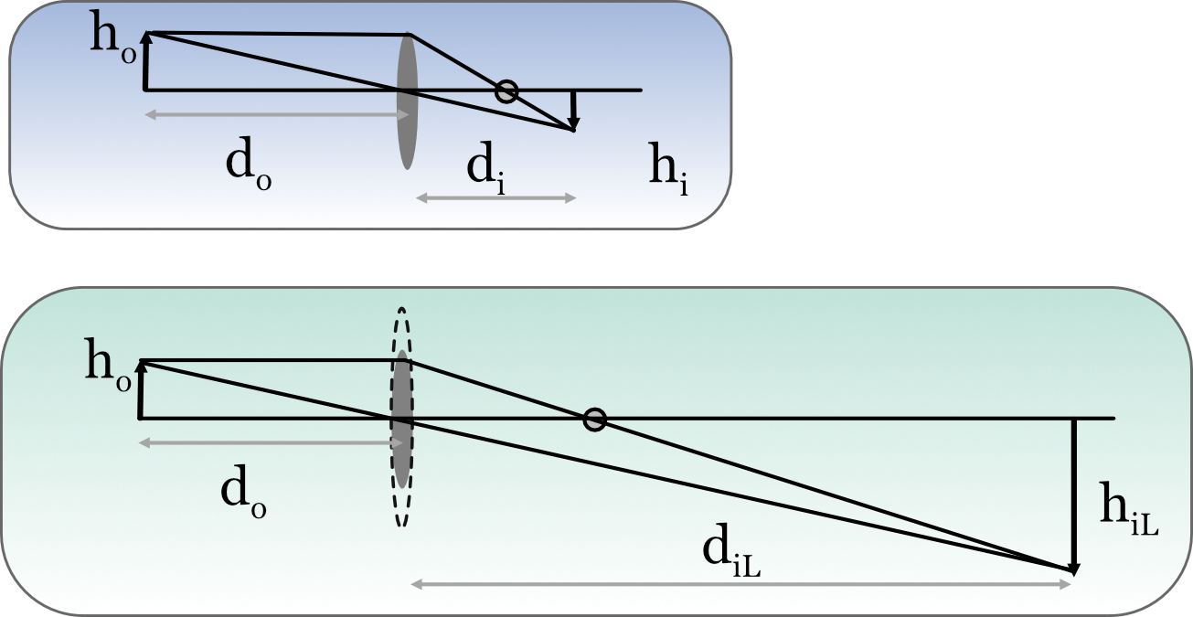
Using the lens formula, the image distance for the lens in the bluish box is
\[ d_i = \frac{f \times d_o}{d_o - f} = \frac{0.1 \times 0.3}{0.3 - 0.1} = 0.15 m \]
The image distance for the lens in the greenish box, with twice the focal length, \(f' = 0.2m\), is
\[ d_{iL} = \frac{0.2 \times 0.3}{0.3 - 0.2} = 0.60 \text{m} \]
The image distance and image size both increase by a factor of \(4\). The two lenses have the same entrance aperture, so they capture the same amount of light. Because the longer focal length lens spreads the image over a larger area, the amount of light per unit area (irradiance) in the image is reduced.
Some camera optics have an adjustable focal length, and this enables the user to adjust the image magnification. The image sensor size, however, is usually fixed. Thus, if we increase the image magnification, the fixed sensor captures a smaller portion of the image, but with the same sensor spatial resolution. The effect is to produce an image that appears to zoom into a portion of the image. This technique, called optical zoom is very effective as long as there is no loss of spatial resolution in the magnified image.
9.14 \(\mathrm{f}/\#\) and image intensity
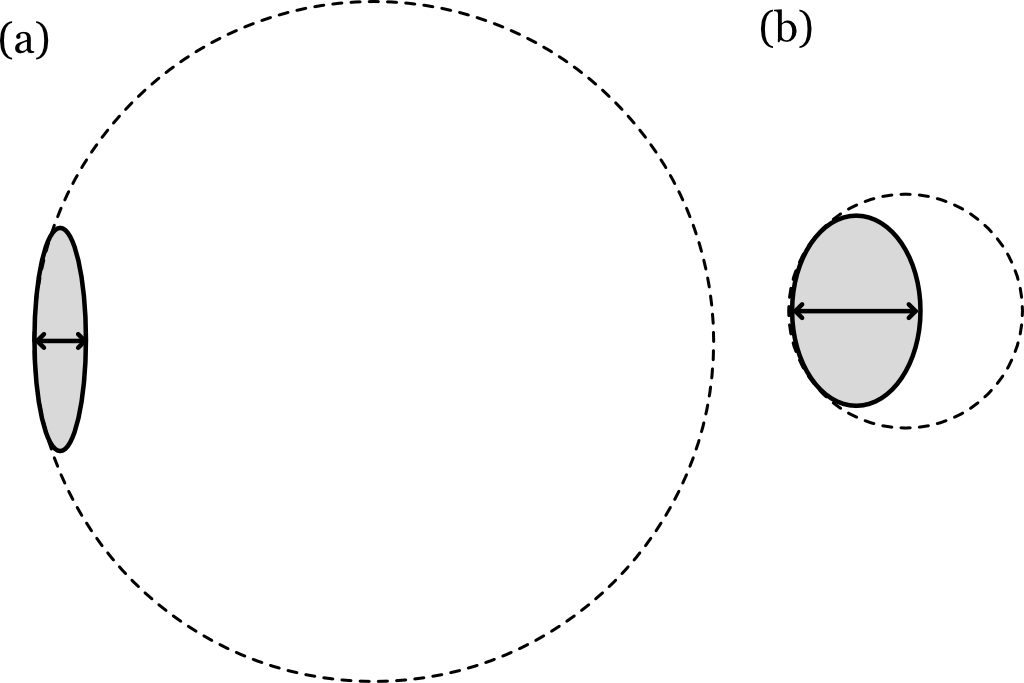
Suppose we wish to magnify the image, but we want to maintain the image irradiance level. In that case, we must capture \(4\) times as much light. We do this by increasing the lens diameter, \(D\). The formula for the area of the aperture is \(\pi (D/2)^2\); thus, doubling the diameter, \(D\), increases the area by a factor of \(4\).
The size of the lens with the larger diameter is sketched by the dashed ellipse in the green section of Figure 9.10. Increasing the focal length expands the image size and reduces the image intensity. Increasing the lens diameter compensates for the reduced intensity. Doubling the focal length and entrance diameter preserves the f/# (ratio of the focal length and the aperture diameter). This example illustrates that lenses with the same f/# produce images with the same image intensity.
9.15 Depth of field
Equation 9.3 tells us how to set the distance between the optics and image plane, \(d_i\), to bring an object at distance \(d_o\) into focus. We might also be interested to answer the related question: Given that an object at \(d_o\) is in focus, what will the blur be for objects nearer or further? The range of distances over which the objects remain in good focus is called the depth of field.
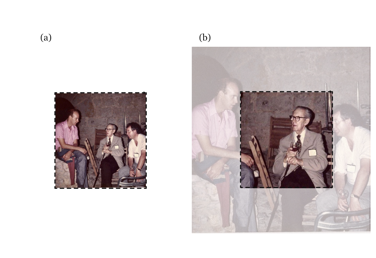
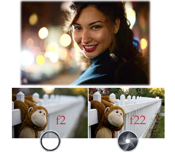
The size of the depth of field can be controlled by adjusting the size of the lens aperture. As it becomes smaller, the lens becomes closer to a pinhole, the depth of field increases. The depth of field can become quite narrow for a large aperture. Controlling the depth of field can create visually interesting images (Figure 9.12). Photographers and cinematographers often use settings to bring the main object of interest into good focus and blurring the rest. The depth of field is a quantitative description of the lens setting. Photographers use the term bokeh to describe the aesthetic impact one can achieve by adjusting the depth of field. This quality depends on the optics as well as the scene contents.
9.15.1 Circle of confusion
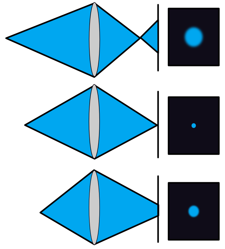
Consider an image formed with a thin lens that is kept at a fixed distance from the image plane (Figure 9.13). The middle image panel shows an object in excellent focus, and the other two panels show points that are too near or too far. As the point moves away from the in-focus object distance, in either direction, the image will be a roughly circular region increases in diameter. This is the circle of confusion. It is a useful concept that is specifically helpful for understanding and quantifying the depth of field.
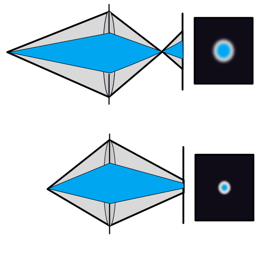
Notice that narrowing the aperture reduces the angle of the rays that arrive at the sensor (Figure 9.14). As the angle narrows, the image size of an out-of-focus point shrinks. If the point is already in focus, however, the rays are arriving at the same point and the image size is little changed. This is the same idea we observed in Section 7.3 when we explained pinhole cameras. This diagram makes clear that a pinhole camera has a very large depth of field. No Bokeh for the pinhole afficianados!
We can use the diameter of the circle of confusion to quantify the depth of field. The diameter depends on the parameters of the lens and image plane (Figure 9.15). The size of the circle of confusion is computed by the ISETCam function opticsCoC.
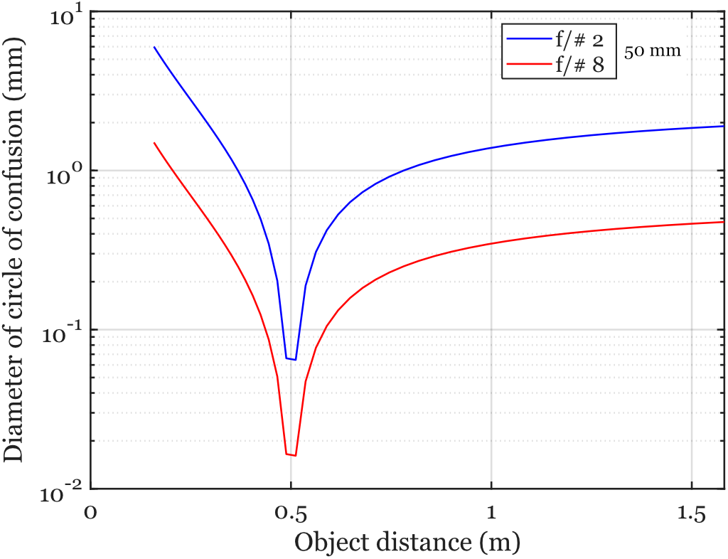
Suppose we select a circle of confusion diameter that we consider to be good focus. From the curves in Figure 9.15, the depth range of good focus will be relatively narrow for the large aperture compared to the small aperture.
The diameter of the circle confusion can be calculated using this geometry. Suppose the image plane is placed so that a point \(P\) is in focus, so that the distance to the image plane is \(f_P\). Another point, \(X\), is closer and thus its focus would be beyond the image plane, say at \(f_X\).
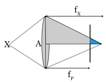
There will be two similar right triangles. One is formed with the sides \(A/2\) (half the aperture) and \(f_X\); the similar triangle (blue) has sides \(f_X - f_P\) and \(C_r\) (the radius of the circle of confusion). Because the right triangles are similar, the sides must satisfy \[ \frac{C_r}{A/2} = \frac{f_X - f_P}{f_X} \]
The diameter of the circle of confusion is twice the radius, \(C = 2*C_r = A \frac{f_X - f_P}{f_X}\)
9.15.2 Depth of field formula
The depth of field formula quantifies the range of object distances that appear acceptably sharp in an image. It is widely used as an approximation, as we approximate an optical system as a thin lens:
\[ \text{DOF} \approx 2 N C ({\frac{d_o}{f}})^2 \tag{9.6}\]
where:
- \(N\) is the lens \(\mathrm{f}/\#\) (focal ratio, dimensionless)
- \(C\) is the acceptable diameter of the circle of confusion (in meters)
- \(d_o\) is the object distance (in meters)
- \(f\) is the lens focal length (in meters)
Recall that \(N = f/A\), where \(A\) is the aperture diameter. Substituting this into the formula gives:
\[ \frac{N}{f^2} = \frac{f}{A} \cdot \frac{1}{f^2} = \frac{1}{A f} \]
So, the DOF formula can also be written as:
\[ \text{DOF} \approx \frac{2 C (d_o)^2}{A f} \]
This relationship shows:
- DOF increases with object distance (\(d_o\))
- DOF increases with the allowable circle of confusion (\(C\))
- DOF decreases as aperture diameter (\(A\)) increases (i.e., with a larger aperture)
- DOF decreases as focal length (\(f\)) increases
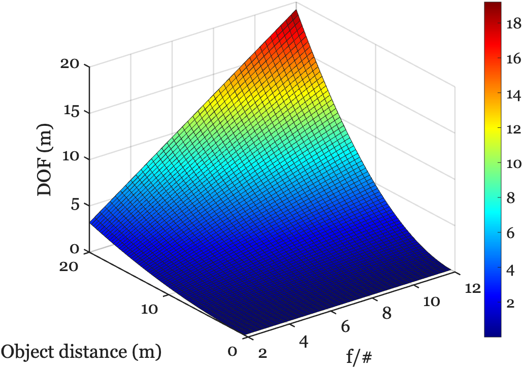
Example:
The plot below shows the DOF for a 100 mm focal length, diffraction-limited lens, as a function of \(\mathrm{f}/\#\) and object distance. The calculations use the ISETCam script s_opticsDoF, which calls opticsDoF to implement Equation 9.6.