29 Linear systems
The book is still taking shape, and your feedback is an important part of the process. Suggestions of all kinds are welcome—whether it’s fixing small errors, raising bigger questions, or offering new perspectives. I’ll do my best to respond, but please keep in mind that the text will continue to change significantly over the next two years.
You can share comments through GitHub Issues.
Feel free to open a new issue or join an existing discussion. To make feedback easier to address, please point to the section you have in mind—by section number or a short snippet of text. Adding a label characterizing your issue would also be helpful.
Last updated: November 17, 2025
29.1 Linear systems overview
Linear systems theory is a foundational topic in science, engineering, and mathematics. Each discipline field explains the importance of linear systems a bit differently, and they use it at varying levels of depth. In this appendix I introduce the core ideas of linear systems for image systems engineering. I have two goals. First, I hope to provide readers an accessible and intuitive description from the point of view of image systems engineering. Second, I will introduce the general notation used throughout this book. My hope is that both newcomers and those with prior exposure will find this chapter a useful reference for the concepts and tools we use in image systems engineering.
29.2 Superposition and Homogeneity
A system \(L\) is linear if it satisfies the superposition rule:
\[ L(x + y) = L(x) + L(y). \tag{29.1}\]
Here, \(x\) and \(y\) are two possible inputs, and \(L(x)\) is the system’s response to the input \(x\). The input variable can be a scalar, vector, matrix, or tensor. For example, in an optical system, \(x\) might represent the incident light field at the entrance aperture, and \(L(x)\) could be the spectral irradiance measured at the sensor. For modeling an image sensor, \(x\) could be the irradiance at the sensor and \(L(x)\) would be the electrons accumulated in the pixels. For human vision, \(x\) might be the spectral power distribution of the incident light field and \(L(x)\) the photon absorptions in the three types of cone photoreceptors.
Homogeneity is special case of superposition:
\[ L(\alpha x) = \alpha L(x) \tag{29.2}\]
Homogeneity follows from superposition. For example, adding an input to itself,
\[ \begin{aligned} L(x + x) &= L(2x) \nonumber \\ &= L(x) + L(x) \nonumber \\ &= 2L(x) . \nonumber \end{aligned} \]
Perhaps you can see how this generalizes to any integer \(m\):
\[ L(m x) = m L(x). \]
Homogeneity is also noted as a special case because a system can be homogeneous without being linear. For example the absolute value, \(f(x) = |x|\), and the vector length function
\[ f(\mathbf{x}) = \|\mathbf{x}\|_2 = \sqrt{x_1^2 + x_2^2 + \cdots + x_n^2} \]
are both homogeneous but not linear. The function \(ReLU(x) = \max(0, x)\), widely used in neural networks, is also homogeneous for \(\alpha > 0\) but not linear:
\[ 1 = ReLU(2 + -1) \neq ReLU(2) + ReLU(-1) = 2 + 0. \]
Remembering that such cases exist may be of use to you in the future.
For real-valued systems that obey superposition, homogeneity holds for any rational number. If \(\alpha = \frac{p}{q}\) is rational:
\[ L(\alpha x) = L\left(\frac{p}{q}x\right) = p L\left(\frac{x}{q}\right). \]
Let \(x' = x/q\), so
\[ L(x) = L(q x') = q L(x') \implies L(x') = \frac{1}{q} L(x). \]
Therefore,
\[ L(\alpha x) = p L(x') = p \frac{1}{q} L(x) = \frac{p}{q} L(x) = \alpha L(x). \]
To extend this to all real numbers, continuity and far more extensive proof is required. But how about we just work with the rationals and be engineers for now?
29.3 Discrete linear systems
The ISETCam simulations rely on discrete representations of linear systems.
We convert a continuous stimulus—such as a spatial pattern or a spectrum—by sampling it at a set of points. In general, a continuous signal \(s(x)\) becomes a vector of sampled values, \(\mathbf{s}\), by sampling it at a set of values, \(x_i\). We might write the entries as \(s[x_i]\), where \(i\) is an integer index, or simply \(s[i]\). The square brackets are a reminder that the signal is discretely sampled.
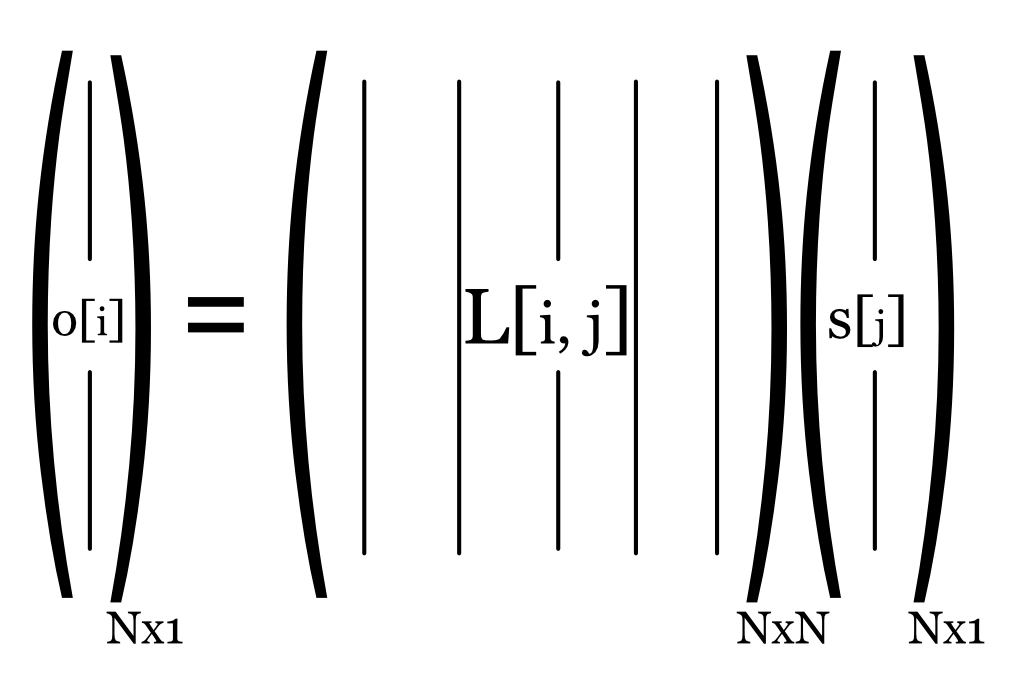
Any discrete linear system can be represented as a matrix, \(\mathbf{L}\), which maps the input vector to an output vector, \(\mathbf{o}\):
\[ \mathbf{o} = \mathbf{L} \mathbf{s} \tag{29.3}\]
This can also be written as a summation:
\[ o[i] = \sum_j L[i,j] s[j] \tag{29.4}\]
It’s helpful to visualize this as a matrix tableau: each column of \(\mathbf{L}\) is scaled by the corresponding entry in \(\mathbf{s}\), and the output vector is the sum of these scaled columns.
Some matrices have an inverse, and for these we can estimate the input by measuring the output. Square matrices are particularly simple to work with, and a square matrix means we are matching the sample spacing of the inputs with the sample spacing of the outputs. Some matrices are not invertible, and the best we can do from the measurements is constrain the set of possible inputs.
The notation we use for the vectors and matrices may vary—sometimes the input is naturally an image (a matrix), and we “flatten” it into a vector; other times, we use tricks to keep the image structure intact and still carry out the computation. But the key idea is always the same: in the discrete world, linear systems are matrices that map input vectors to output vectors.
Throughout this volume, I am trying to keep the mathematical typography consistent with this table.
| Notation | Meaning |
|---|---|
| Bold capital letter (\(\mathbf{B}\)) | Matrix |
| Bold lower case (\(\mathbf{s}\)) | Vector (column, \(N \times 1\)) |
| Ordinary lower case (\(\alpha\), \(s\)) | Scalar (Latin or Greek) |
| Ordinary upper case (\(L(u,v)\)) | 2D matrix or image (continuous) |
| \(L[\text{row},\text{col}]\) | Discrete image or matrix (row, col ordering) |
| \(\mathbf{B^t}\) | Matrix or vector transpose (superscript \(t\)) |
29.4 Pointspread matrix
Image systems engineers often examine system performance by measuring the response to a point of light—this is the point spread function (PSF) introduced in Section 7.8. A point of light, \(p_i\), is represented by a vector that has \(1\) in a single location and zeros elsewhere. Each column of the linear transformation, \(\mathbf{L}\), is the point spread function corresponding to the sampled point, \(\text{PSF}_i\).
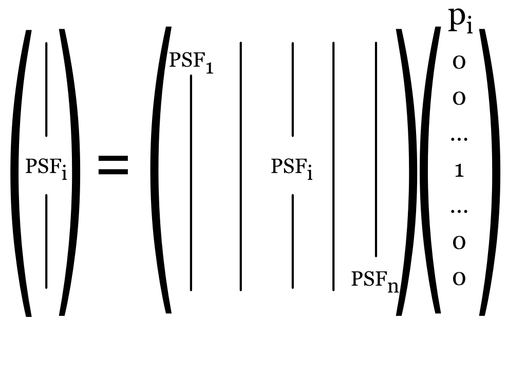
I drew this tableau for a one-dimensional point spread, to make the idea clear. For two-dimensional images, we would have to flatten the image data into columns. But only complexity would be added, and the principles would be unchanged.
29.5 Spatial basis functions
The PSF is a fundamental tool, but it has limitations: using a point of light involves very few photons, and PSFs can vary in complex ways that are hard to summarize with just a few parameters. A key insight is that we can use linear models to describe images in many different ways, not just as a collection of points. Some alternative representations are especially useful for analyzing the optical performance of imaging systems. Here, we use linear models to create alternative representations of the spatial intensity of images, \(S[u,v]\).
A linear model for spatial intensity looks like this:
\[ S[u,v] = \sum_{i} w[i] B_i[u,v] \tag{29.5}\]
The functions \(B_i[u,v]\) are called spatial basis functions, and the scalars \(w[i]\) are the weights for each basis function. The image intensity \(S[u,v]\) is just a weighted sum of these basis functions.
If we agree on a set of basis functions, then we can describe any image simply by specifying the weights. In fact, when we describe an image as a grid of intensity values, we’re implicitly using a set of point basis functions—each one nonzero at a single location and zero everywhere else.
29.6 Image transforms
For a linear model to be useful, we need a way to find the basis weights from the image. A function that maps an image, \(S[u,v]\) to the weights \(w[i]\) is called an image transform. If we choose orthonormal basis functions this transform becomes especially simple. Define the inner product \[ \langle A, B \rangle \;=\; \sum_{u,v} A[u,v]\;B[u,v]. \] Orthonormal means \[ \langle B_i, B_j \rangle \;=\; \begin{cases} 0, & i \ne j \\ 1, & i=j \end{cases} \tag{29.6}\]
To work with these two-dimensional images mathematically, we often “flatten” each basis function \(B_i\) (which is a matrix) into a long column vector by stacking its columns. We do the same for the image \(S[u,v]\), turning it into a vector \(\mathbf{s}\). If we collect all the basis vectors into the columns of a matrix \(\mathbf{B}\), and the weights into a vector \(\mathbf{w}\), we can write the linear model from Equation 29.5 as a matrix equation:
\[ \mathbf{s} = \mathbf{B w} \tag{29.7}\]
Here, the \(i^{th}\) entry in \(\mathbf{w}\) multiplies the \(i^{th}\) column of \(\mathbf{B}\), and the sum gives us the image vector \(\mathbf{s}\). This is just a compact way of writing the weighted sum from before.
Now, if the basis functions are orthonormal, then \(\mathbf{B^t B}\) is the identity matrix. This makes it easy to recover the weights from the image:
\[ \begin{aligned} \mathbf{s} &= \mathbf{B w} \\ \mathbf{B^t s} &= \mathbf{B^t B w} \\ \mathbf{B^t s} &= \mathbf{w} \end{aligned} \tag{29.8}\]
In words: just multiply the image vector by the transpose of the basis matrix to calculate the weights. If the basis functions are orthogonal but not normalized, replace \(\mathbf{B^t}\) by \((\mathbf{B^t B})^{-1}\mathbf{B^t}\).
This seems almost too trivial to mention. But here we go.
When we describe images as points, \(S[u,v]\), we are implicitly using the point basis. The point basis functions are zero everywhere except at a single location: \[ B_{m,n}[u,v] \;=\; \begin{cases} 1, & (u,v)=(m,n) \\ 0, & \text{otherwise.} \end{cases} \]
With this basis, the weights are simply the image intensities, and the expansion is \[ S[u,v] \;=\; \sum_{m,n} S[m,n]\; B_{m,n}[u,v]. \tag{29.9}\]
Because each \(B_{m,n}\) is nonzero at only one location, the basis is orthonormal under the discrete inner product, and the matrix formed by stacking the basis vectors is the identity.
29.7 Eigenfunctions
An eigenfunction (or, in the discrete case, an eigenvector) of a system is a special input that produces an output that is simply a scaled version of itself. In other words, when you feed an eigenfunction into a linear system, the system just scales it—nothing else changes. This property is incredibly useful, because it means we can predict exactly what will happen to these inputs.
For a discrete linear system represented by a matrix \(\mathbf{L}\), a column vector \(\mathbf{e}_i\) is an eigenvector if
\[ \mathbf{L} \mathbf{e}_i = \alpha_i \mathbf{e}_i \tag{29.10}\]
where \(\alpha_i\) is the eigenvalue associated with \(\mathbf{e}_i\). The eigenvalue tells us how much the eigenvector is stretched or shrunk by the transformation.
Many image systems we describe in this book have a complete set of orthogonal eigenvectors. By a complete set, I mean (a) the eigenvectors of the system are a basis for the input (Section 29.5), and (b) the eigenvectors are orthogonal to one another (Section 29.6). This means we can express any input vector (stimulus) as a weighted sum of the image system’s eigenvectors. The power of this observation is that measuring the system response to an eigenvector input is very simple:
\[ \begin{aligned} \mathbf{o} & = \mathbf{L} \mathbf{s} \\ & = \mathbf{L} \left(\sum_i \sigma_i \mathbf{e}_i \right) \\ & = \sum_i \sigma_i \mathbf{L} \mathbf{e}_i \\ & = \sum_i \sigma_i \alpha_i \mathbf{e}_i \end{aligned} \tag{29.11}\]
Here, \(\mathbf{s}\) is the input, written as a sum of eigenvectors with weights \(\sigma_i\). The output \(\mathbf{o}\) is just the sum of the same eigenvectors, but now each one is scaled by its eigenvalue \(\alpha_i\). This makes analyzing and understanding the system much easier.
Not all linear systems have a complete set of eigenvectors. Only discrete linear systems represented by normal matrices are guaranteed to have an orthogonal set of eigenvectors. The definition of a normal matrix is1.
\[ \mathbf{L L^* = L^* L} . \tag{29.12}\]
29.8 Local linearity
No real system is linear for all possible inputs. If you push a system with extremely large signals—say, by shining a laser into a camera or overloading an amplifier—it may behave unpredictably or even break! But for most practical purposes, many systems are linear over a useful range of inputs.
When a system is not linear everywhere, it may still be well-approximated as linear within a limited region of its input space. In other words, the system is locally linear: if you keep your signals similar enough to a particular operating point, the system’s behavior is linear, even if it isn’t globally so.
For a locally linear system, the best linear approximation depends on where you are in the input space. The linear model near \(x_1\) might look quite different from the linear model near \(x_2\). So, when modeling or analyzing a locally linear system, it’s important to know which region you’re working in.
In practice, the optics of most imaging systems are linear over a large range, but they are shift-invariant over a smaller input range, only within a limited region of the field of view. This is called local shift invariance. Such a region is known as an isoplanatic patch. The shift-invariant analysis applies well to such local regions, and degrades if we measure over larger regions.
This principle of local linearity, or local shift-invariance, is fundamental in mathematics, physics, and engineering.2 It’s the reason why linear models are so widely used, even for systems that aren’t truly linear everywhere.
The \(*\)-operator means conjugate transpose. This means take the complex conjugate of each entry (\(a + ib \rightarrow a - ib\)), and transpose the matrix. For a real matrix, the \(*\)-operator amounts to the usual matrix transpose.↩︎
If you’ve seen the Taylor series expansion in calculus, you’ve already encountered local linearity. Near a point \(x\), you can approximate a function by its value at \(x\) plus a correction that depends on how far you are from \(x\) and the derivative at \(x\).↩︎