10 Lenses and ray transfer
The book is still taking shape, and your feedback is an important part of the process. Suggestions of all kinds are welcome—whether it’s fixing small errors, raising bigger questions, or offering new perspectives. I’ll do my best to respond, but please keep in mind that the text will continue to change significantly over the next two years.
You can share comments through GitHub Issues.
Feel free to open a new issue or join an existing discussion. To make feedback easier to address, please point to the section you have in mind—by section number or a short snippet of text. Adding a label characterizing your issue would also be helpful.
Last updated: November 2, 2025
10.1 Lenses and ray transfer overview
The principles of geometric optics and thin lenses are also critical for thick lenses and multi-element lenses(Chapter 7). The first lens is traced, and its output is the input to a second lens. We can use the three principles (Section 9.5) to analyze the lenses in sequence. Using these tools, but with increasing complexity, the methods used to characterize thin lenses (Chapter 9) can be extended to many different optical functions.
In this chapter, I will illustrate some of the extensions to thick lenses and multi-element lenses. These have been important historically, and they will continue to be with us for some years.
But let’s start here, with increasingly complex optics.
10.2 Combining two thin lenses
Let’s take a simple step towards more complex optical systems by combining two thin lenses. When we place two lenses in series, the image formed by the first lens becomes the object for the second.
If the lenses have focal lengths \(f_1\) and \(f_2\) and are separated by a distance \(d\), the effective focal length (\(f\)) of the combination is given by:
\[ \frac{1}{f} = \frac{1}{f_1} + \frac{1}{f_2} - \frac{d}{f_1 f_2} \tag{10.1}\]
This formula gives the focal length of an equivalent single thin lens. However, it’s important to remember that this equivalent lens isn’t located at the position of either of the original lenses. Its position is defined by the system’s principal planes, which we’ll discuss more in the context of thick lenses.
Recalling that the power of a lens (in diopters) is the inverse of its focal length, Equation 10.1 shows that: * When the lenses are touching (\(d \approx 0\)), their powers simply add up: \(P = P_1 + P_2\). * As the lenses are separated, the total power changes. If \(d = f_1 + f_2\), the total power becomes zero (\(f = \infty\)). This specific arrangement is called a focal telescope, and it collimates light, meaning parallel incoming rays emerge as parallel outgoing rays.
A more practical value is the back focal length (BFL), which is the distance from the back surface of the last lens to the system’s final focal point. For our two-lens system, this is:
\[ \text{BFL} = \frac{f_2 (d - f_1 )}{d - (f_1 + f_2)} \tag{10.2}\]
The BFL tells you exactly where to place a sensor to capture a sharp image of an object at infinity. Notice that when \(d = f_1 + f_2\), the denominator is zero, and the BFL becomes infinite, which is consistent with the parallel rays produced by a focal telescope.
10.3 Thick lens definitions
The principles of refraction and ray tracing apply to both thin and thick lenses. However, for a thick lens, the optical design calculations must account for the distance rays travel within the lens material. This internal propagation distance is assumed to be zero in thin lens calculations, which is a key simplification.
We can extend the three principles used for thin spherical lenses (Section 9.5) to analyze thick lenses. The concept of the focal point remains the same: Rays arriving parallel to the optical axis converge toward the image-side focal point (\(F_2\)). Conversely, rays passing through the object-side focal point (\(F_1\)) emerge parallel to the optical axis.
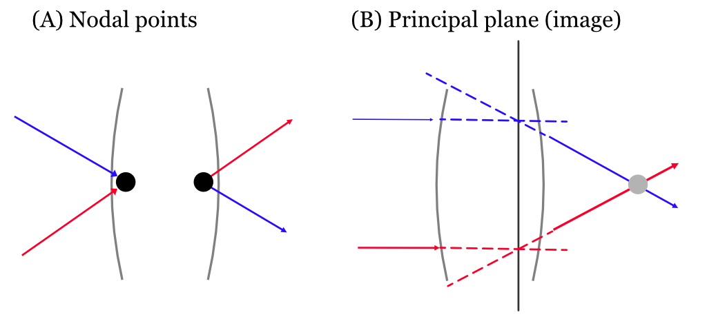
For a thin lens, we noted that a ray passing through the optical center is undeviated. A thick lens has a similar concept, but it involves two nodal points (\(N_1\) and \(N_2\)). A ray directed toward the object-side nodal point (\(N_1\)) emerges from the lens as if it came from the image-side nodal point (\(N_2\)), traveling parallel to its original direction (Panel A, Figure 10.1).
To handle the ray’s path, it is also convenient to define two principal planes (\(P_1\) and \(P_2\)). Consider rays parallel to the optical axis entering the lens. They exit the lens converging toward the focal point. If we extend the incoming parallel ray forward and the outgoing converging ray backward, they intersect. The locus of these intersection points for rays near the optical axis forms the image-side principal plane, \(P_2\) (Panel B, Figure 10.1). A similar construction using rays from the front focal point defines the object-side principal plane, \(P_1\). The intersection of a principal plane with the optical axis is called a principal point.
In the general case, a thick lens is characterized by six cardinal points: two focal points, two principal points, and two nodal points. However, in the common situation where the medium on both sides of the lens is the same (e.g., air), the nodal points coincide with the principal points. This simplifies the system considerably (Figure 10.2).
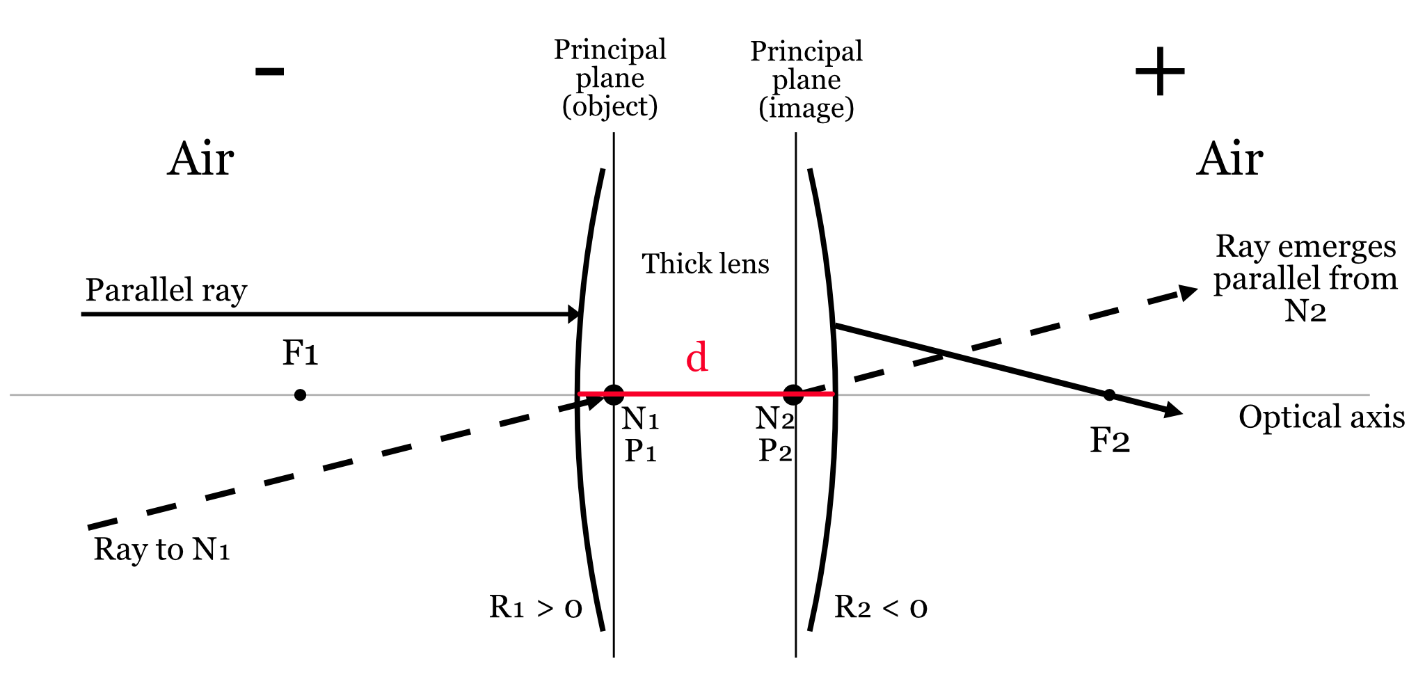
Just as the thin lens has a lensmaker’s formula (Equation 9.4), a similar equation exists for a thick spherical lens to calculate its effective focal length:
\[ \frac{1}{f} = (n - 1) \left ( \frac{1}{R_1} - \frac{1}{R_2} + \frac{(n - 1) d}{n R_1 R_2} \right ) \tag{10.3}\]
Here, \(n\) is the refractive index of the lens material relative to the surrounding medium, \(d\) is the lens thickness, and \(R_1\) and \(R_2\) are the radii of curvature of the two surfaces. The formula differs from the thin lens version by an extra term that accounts for the lens thickness, \(d\).
While this formula works for a single thick lens, applying it repeatedly for a multi-element system becomes unwieldy. A more powerful and systematic approach uses matrix multiplication, which I will introduce after we discuss multi-element lenses.
10.4 Multi-element thick lenses
The ray tracing principles developed so far are the foundation for the next level of complexity, analyzing combinations of thick lenses. If one has a set of thick lenses in combination, each can be represented by a pair of principal planes. The next step is to combine this pair into a new, single pair, that specifies them jointly. One then continues along this path, adding in new lenses, taking into account various details such as magnification. (J&W page 93).
Doing this analysis by hand, and using the various formulae, can be quite difficult. The rise of optical design software tools made it possible for many people to engage in the task. Understanding the principles is important for using these software tools well.
But even before these tools were available, there was great interest in designing useful optics. For example, the development of photography, such as daguerrotype in 18391, created a significant market for optical design. People wanted to take pictures of themselves, their family, and their friends. The low light sensitivity of the recording media made it difficult to create portraits using a pinhole camera. Also, the pinhole camera does not produce a flat field image (Section 7.2.1). Lens designers set out to make portraits possible. Much of this was enabled by the development of new types of glass with different optical properties, especially from Fraunhofer’s work in Bavaria (Section 5.2). Having a palette of materials to use made the design possible.
The development of mathematical methods for predicting the outcome for lenses with different shapes and materials was also important. Both Gauss and Petzval were mathematicians who developed workable methods for simulating the impact of a design prior to construction. Robert Wood, an American physicist, coined the term “fish-eye” lens to describe how a fish would see the world through a 180° hemisphere of water2. He designed a lens to mimic this — essentially a hemispherical objective producing a circular image. For all of those designers, mathematics was the key simulation tool. In the modern era, as this book illustrates in many places, mathematics is extended into computable algorithms. These are our modern tools, but don’t sleep on the importance of mathematics!
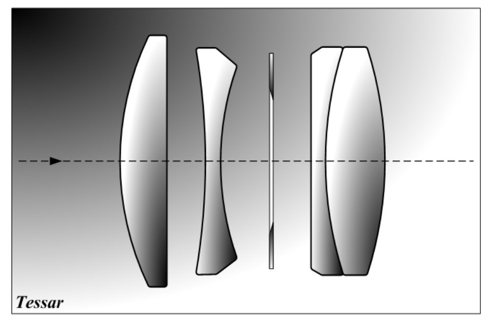
Finally, in those days like these, different design goals led to diversity. Gauss was primarily interested in astronomical lenses with low distortion. Petzval proritized light sensitivty for portraiture. Cooke (1893) later produced the famous triplet, which became the Tessar, to achieve a compact lens that balanced aberrations across the field. Woods’ fish-eye became a scientific tool that enabled measurements of the sky, military reconnaissance and artistic architectural overviews.
10.4.1 Double Gauss
The great mathematician Gauss implemented proposed a design, the Gauss lens for astronomy. This was improved upon by Alvan Clark and Paul Rudolph, who expanded on Gauss’s idea to introduce the first symmetrical double Gauss arrangement — essentially two of Gauss’s lens pairs, placed symmetrically around the stop . Paul Rudolph at Zeiss refined this into the famous Planar lens (1896), which became the archetypal “double Gauss” photographic objective. This design, with later improvements (e.g. Taylor & Hobson’s Opic lens, 1920), became the dominant fast normal lens type for photography in the 20th century (Figure 10.3).
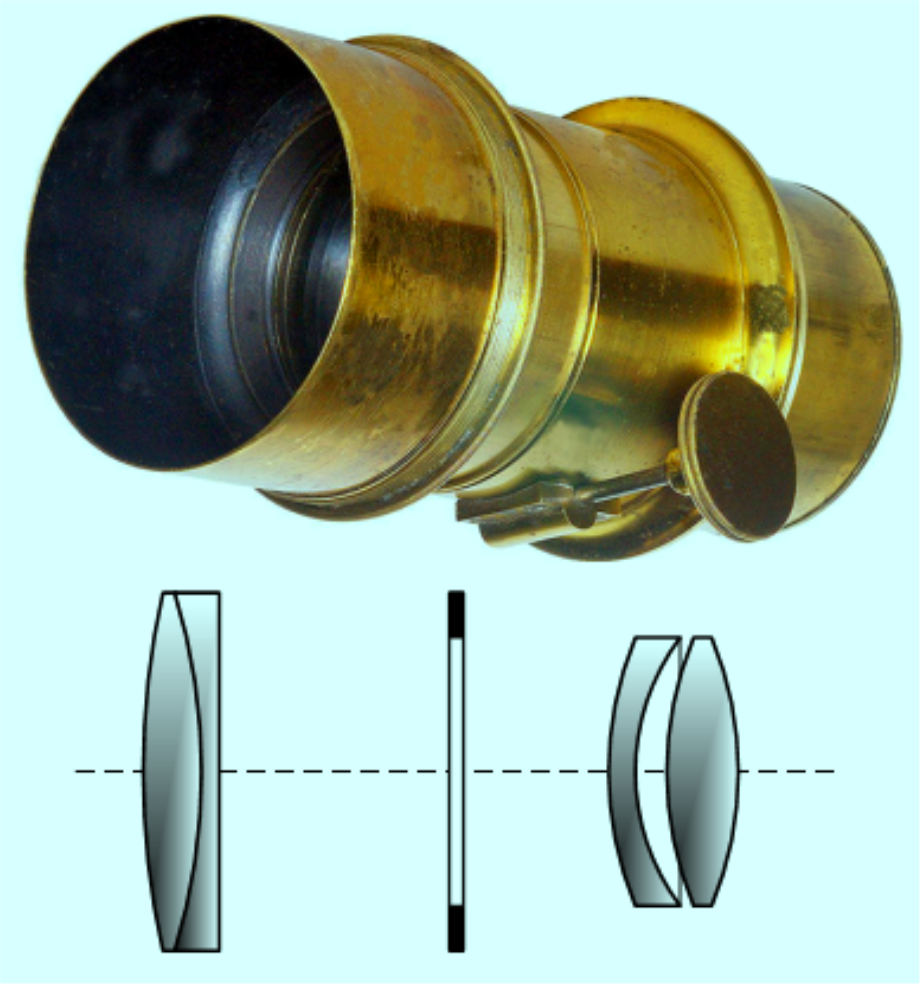
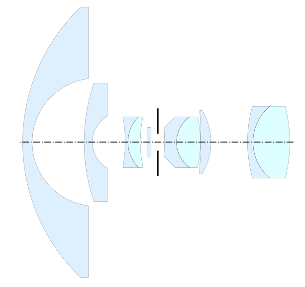
10.4.2 Tessar, Petzval and Fisheye
The three tabs in the image below illustrate the Tessar, Petzval and Fisheye designs. As you can imagine from inspecting these lens diagrams, there is a large university of shapes, spacing, and materials that were open for exploration. As you might also imagine, the ability to search through this space with a goal in mind, and with increasingly large computers and purpose-built software to compute the properties of the optics, has been important to image systems engineering.
10.5 ABCD matrix optics
Ray tracing provides a physical and intuitive way to understand how light travels. But the method becomes computationally intensive for complex systems with many surfaces. A powerful and systematic method for analyzing such systems is ray transfer matrix analysis, often called ABCD matrix optics. This approach simplifies the design process by modeling the effect of each optical component on a light ray using a simple \(2 \times 2\) matrix.
This method is accurate for paraxial rays; these are rays that are both close to the optical axis and travel at small angles relative to it. The accuracy of the method depends on these small-angle approximations:
\[ \sin(\theta) \approx \theta, \quad \tan(\theta) \approx \theta, \quad \cos(\theta) \approx 1 \]
These approximations are accurate for angles up to about \(5^\circ\) and can often be stretched to \(10^\circ\) depending on the required accuracy. They also apply to rays that are one-third to one-half of the aperture distance, depending on the lens power.
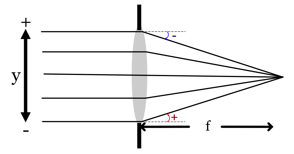
A paraxial ray at any point along the optical axis can be described by a vector containing two values: its radial distance (\(y\)) from the optical axis and its angle (\(\theta\)) with respect to the axis.
We represent the ray as a column vector, \(\rho = \begin{pmatrix} y \\ \theta \end{pmatrix}\). The journey of this ray through an optical system is described by a series of matrix multiplications, where each matrix represents a single optical element (like a lens surface) or the space between elements. The final output ray \(\rho_{\text{out}}\) is found by applying the total system matrix \(M\) to the input ray \(\rho_{\text{in}}\):
\[ \rho_{\text{out}} = M \rho_{\text{in}} \quad \text{or} \quad \begin{pmatrix} y_{\text{out}} \\ \theta_{\text{out}} \end{pmatrix} = \begin{pmatrix} A & B \\ C & D \end{pmatrix} \begin{pmatrix} y_{\text{in}} \\ \theta_{\text{in}} \end{pmatrix} \]
Let’s build the matrices for a thick lens by following a ray as it refracts at the first surface, travels through the lens material, and refracts again at the second surface.
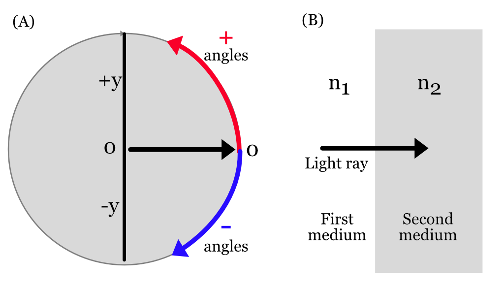
10.5.1 Refraction - First Surface
Snell’s Law tells us how the rays change direction at the first surface of a spherical lens (Equation 8.1). As you can see in Figure 10.6, the rays change direction by an amount that depends on their field height. The critical point -I won’t show the derivation- is that the amount of change is proportional to field height. In the paraxial regime the change is the same, no matter what the input ray angle.
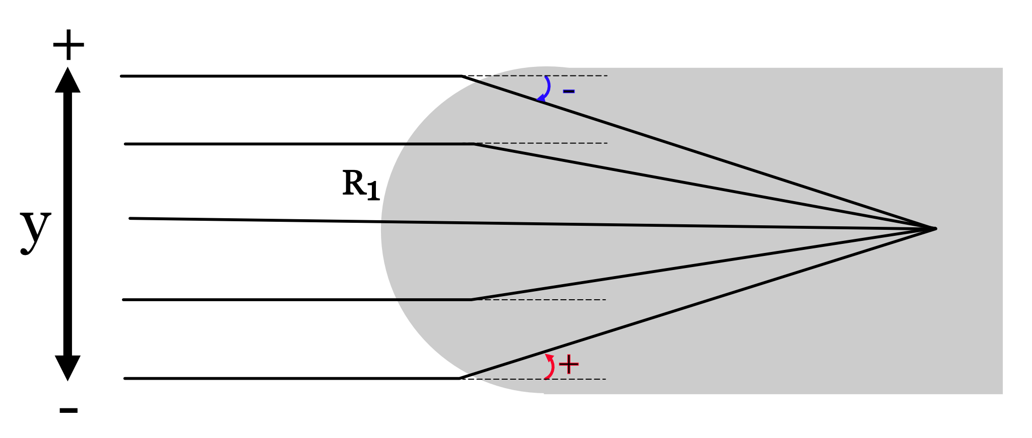
As the ray passes through the surface, the field height itself does not change. We can use these two observations to create the ray transfer matrix that describes how the input ray, \(\rho_1 = (y_1, \theta_1)\) becomes the output ray, \(\rho_2\).
\[ M_{S1} = \begin{pmatrix} 1 & 0 \\ \dfrac{n_1 - n_2}{R_1 ~ n_2} & \dfrac{n_1}{n_2} \end{pmatrix} \qquad \rho_2 = M_{\text{S1}} \rho_1 \]
where:
- \(n_1\) is the refractive index of the medium on the left (e.g., air),
- \(n_2\) is the refractive index of the lens material,
- \(R_1\) is the radius of curvature of the first surface (positive for convex, negative for concave).
10.5.2 Translation Through the Lens
After a light ray crosses a surface boundary, it continues in a straight path. In this case, the situation is reversed: the field height \(y\) changes but the angle (direction) does not. The change in field height is proportional to the angle, \(y = d \theta\). This makes the ray transfer matrix through a uniform medium quite simple. \[ M_{T} = \begin{pmatrix} 1 & d \\ 0 & 1 \end{pmatrix} \]
10.5.3 Refraction - Second Surface
Finally, as the ray passes the second surface into the surrounding medium, we have a ray transfer matrix with different parameters but the same structure as the first surface.
\[ M_{S2} = \begin{pmatrix} 1 & 0 \\ \dfrac{n_2 - n_1}{R_2 n_1} & \dfrac{n_2}{n_1} \end{pmatrix} \]
where:
- \(R_2\) is the radius of curvature of the second surface,
- \(n_2\) is the refractive index inside the lens,
- \(n_1\) is the refractive index of the medium outside the lens.
These three matrices describe the ray’s journey. Their product is the ray transfer matrix of the entire thick lens. The \(2 \times 2\) matrix \(M\) is called the ABCD matrix,
\[ M = \begin{pmatrix} A & B \\ C & D \end{pmatrix} = M_{S2} M_{T} M_{S1} \]
If we have optics with more spherical, circularly symmetric surfaces, we can continue to define and apply more matrices to create the ray transfer matrix for the system. We only need to know the indices of refraction and the radii of curvature of each surface. If the lenses are close to spherical near the optical axis, this approach still serves as an approximation of performance.
A useful special case to remember is the ray transfer matrix for a thin spherical lens, with the surrounding medium air, \(n_1 = 1\), and the index of refraction of the material is \(n\). This case is a bit simpler because the thickness is considered to be \(d=0\). For a thin lens, the \(y_1\) value of the object side ray is the same as the \(y_2\) on the image side. The angle of the input ray angle, \(\theta_1\), becomes a new angle, \(\theta_2\).
We can calculate the constant of proportionality \(\Phi\) from the lens parameters (indices of refraction and radii of curvature) and medium.
\[ \Phi = \frac{n_{2}-n_{1}}{n_{1}} \left(\frac{1}{R_{1}} - \frac{1}{R_{2}}\right) \tag{10.4}\]
We can express the transformation of the ray \((y_1, \theta_1)\) into \((y_2, \theta_2)\) as 2x2 matrix, accounting for the sign convention,
\[ M_{\text{lens}} = \begin{pmatrix} 1 & 0 \\ -\Phi & 1 \end{pmatrix}, \]
That’s cool. And for a thin lens, it’s even more cool because really only the focal length really matters. Imagine what happens if the focal length shortens (the angles increase) or lengthens (the angles decrease). In fact we can express the focal length \(f\) in terms of the lens parameters this way.
\[ \frac{1}{f} = \left(\frac{n_{2}}{n_{1}} - 1\right) \left(\frac{1}{R_{1}} - \frac{1}{R_{2}}\right), \tag{10.5}\]
so the thin lens matrix can also be written this way
\[ M_{\text{lens}} = \begin{pmatrix} 1 & 0 \\ -\tfrac{1}{f} & 1 \end{pmatrix}. \]
10.5.4 Effective and back focal lengths
Multi-lens systems can be summarized by their ray transfer matrix. This is a very efficient way to communicate about system properties, though it is quite incomplete compared to a full specification of the components and their materials. Because the lens element are not part of the specification, the this characterization of the lens is often called a black box model of the optics. We know what it does, just not how it does it.
We can compute two particularly valuable system properties from the system matrix: the back focal length (BFL), \(f_B\), and the effective focal length (EFL), \(f_E\). The BFL is the distance from the system’s output reference plane to the focal point (for an object at infinity). The EFL is the distance from the secondary principal plane to the focal point.
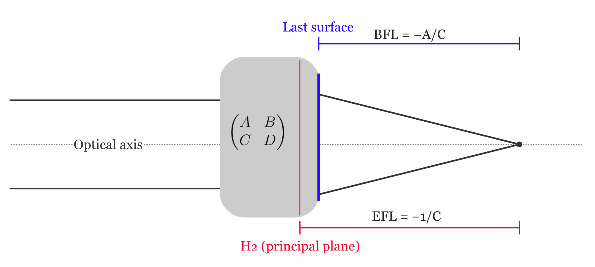
We determine these focal lengths from the system matrix. We compute where an input ray that is parallel to the optical axis emerges and crosses the optical axis. An input ray parallel to the optical axis has the form \(\rho_{\text{in}}=(y_{\text{in}},\theta_{\text{in}})=(y,0)\). Because \(\theta_{\text{in}}=0\), the corresponding output ray depends only on \(A\) and \(C\), \(\rho_{\text{out}}=(y_{\text{out}},\theta_{\text{out}})=(A y, C y)\).
The two output parameters determine the line the output ray follows in the \(z\)-direction. It starts at the output field height and slopes toward the optical axis. The line reaches the optical axis at the \(z\) where \[ \begin{aligned} 0 &= y_{\text{out}} + z\,\theta_{\text{out}} \\ z &= -\frac{y_{\text{out}}}{\theta_{\text{out}}} = -\frac{A}{C}. \end{aligned} \]
By definition of the principal planes, we can shift the reference planes so the system behaves like a thin lens there (this choice makes \(A=1\), while \(C\) is invariant to such shifts). Hence \[ f_{B} = -\frac{A}{C}, \qquad f_{E} = -\frac{1}{C}. \]
N.B. I use a simple parameterization of the ray state, \((y,\theta)\). Others -and they can be very smart- prefer to use the reduced-angle convention. They incorporate the index of refraction into the angle \((y,n\,\theta)\). In that framing, replace \(C\) by \(C/n_{\text{out}}\).
10.6 Ray transfer functions
I expect that we will continue to see computational methods based on rays continue to expand. The ray transfer framing is an important conceptualization and it is thrilling to see the roots of linear algebra and optics coordinate so well. The limitation of the approach to circularly symmetric, paraxial analyses is quite significant. It is clear that we would like to be able to broaden the approach, say by developing functions that map the entire set of input rays to the output rays.
A number of groups have worked to put together functions that extend the ABCD formulation to a much broader mapping, which Goossens et al. (2022) labeled the Ray Transfer Function. Some groups mapped the rays using polynomials (Hopkins, Hullin et al. (2012)), and others have worked with neural networks (Xian et al. (2023)).
The future of lens manufacturing and design is likely to include metalenses (Section 8.6.6) based on nanoscale structures that cannot be modeled by ray training, it will become increasingly important to develop tools to specify the ray transfer function of optical components. The development of this infrastructure is a large, and interesting, task for the future.
An early photographic process employing an iodine-sensitized silvered plate and mercury vapor.↩︎
“In discussing the peculiar type of refraction which occurs when light from the sky enters the surface of still water, it seems of interest to ascertain how the external world appears to the fish. As is well known, a sublnerged eye directed towards the surface of still water sees the sky compressed into a comparatively small circle of light, the centre of which is always immediately above the observer, the appearance being as if the pond were covered with an opaque roof provided with a circular aperture or window. If our eyes were adapted to distinct vision under water, it is clear that the objects surrounding the pond, such as trees, horses, fishermen, etc., would appear round the edge of this circle of light. Objects not much elevated above the plane of the water would be seen somewhat compressed and distorted, but the circular picture would contain everything embraced within an angle of 180 deg in every direction, i.e. a complete hemisphere” Wood (1906)↩︎