30 Linear Space-Invariant (LSI) Systems
The book is still taking shape, and your feedback is an important part of the process. Suggestions of all kinds are welcome—whether it’s fixing small errors, raising bigger questions, or offering new perspectives. I’ll do my best to respond, but please keep in mind that the text will continue to change significantly over the next two years.
You can share comments through GitHub Issues.
Feel free to open a new issue or join an existing discussion. To make feedback easier to address, please point to the section you have in mind—by section number or a short snippet of text. Adding a label characterizing your issue would also be helpful.
Last updated: October 7, 2025
31 Linear Space-Invariant (LSI) Systems overview
Linear models are a cornerstone of science and engineering. For image systems, we can describe these models using different mathematical representations, or basis functions. Two are particularly important.
The first is the point basis, where an image is treated as a collection of individual points (pixels). This is the most intuitive representation. The second is the harmonic basis, which represents an image as a sum of sine and cosine waves of different spatial frequencies.
While the point basis is natural, the harmonic basis is powerful. Harmonics have a special relationship with an important class of systems known as linear space-invariant (LSI) systems: they simplify the analysis enormously. This appendix explains this relationship and introduces the key tools, like the Fourier transform, that are built upon it.
- Linear shift‑invariant (LSI) = linear space‑invariant. “Shift” emphasizes translation; “space” emphasizes domain. We use LSI.
- Point spread function (PSF) = spatial impulse response (response to a Dirac delta, \(\delta[x,y]\)). For time signals the term is impulse response.
- Convolution (circular, length \(N\)): \((I * h)[n] = \sum_{k=0}^{N-1} I[k]\,h\!\big((n-k)\bmod N\big)\). Linear (non‑wrapping) convolution requires zero‑padding (to at least \(N+M-1\)) before using the DFT.
- Correlation vs convolution: convolution flips the kernel; correlation does not. Circular cross‑correlation is \[ R_{x,y}[n] = \sum_{k=0}^{N-1} x[k]\;y\!\big((k+n)\bmod N\big)^{*}, \] using complex conjugation for complex data (drop \({}^*\) for real signals).
- Fourier tools: DFS (series on finite, periodic data), DFT (transform between samples and complex weights), FFT (fast algorithm for the DFT). DTFT/CTFT are infinite‑length/continuous counterparts.
- Sampling and Nyquist: sample pitch \(\Delta x \Rightarrow\) sampling rate \(f_s=1/\Delta x\); Nyquist \(f_N=f_s/2\). Frequencies above \(f_N\) alias (fold) into lower bands. Always state units (e.g., cycles/deg, cycles/mm).
- Boundary conditions: periodic wrap (circular convolution), zero‑padding (linear convolution), or windowing/tapering to control edge artifacts.
31.1 Space-invariance
A practical challenge in characterizing general linear systems is that each input point could have a different point spread function (PSF). That’s a lot to measure! Fortunately, many real systems are much simpler: their PSF is essentially the same, except that it’s shifted to match the shift in input location. In other words, the shape of the PSF doesn’t change—it just translates. We call such systems space-invariant.
Space-invariant linear systems are common across science and engineering. Many physical devices and phenomena can be well-approximated as space-invariant, at least over a useful range. This property makes them much easier to calibrate: we only need to measure a single PSF -the response to a single point!- rather than measure every possible point. You can see why for a space-invariant system the PSF is the key measurement that characterizes the system.
Because space invariance simplifies both analysis and computation, many courses on “linear systems” focus almost entirely on the space-invariant case.
Let’s make the idea of space invariance a bit more precise. Suppose we use \(T()\) to represent a shift (translation) operation. If we shift an image \(x\) by an amount \(\delta\), we write \(T(x, \delta)\). A system \(L()\) is space-invariant if shifting the input and then applying the system gives the same result as applying the system first and then shifting the output (possibly by a scaled amount):
\[ L(T(x, \delta)) \approx T(L(x), \alpha \delta). \tag{31.1}\]
Here, \(\alpha\) is a scale factor that accounts for magnification or other effects. For example, if you move an object by \(\delta\) meters, its image might move by \(\alpha \delta\) meters on the sensor.
31.2 LSI system matrix
An LSI system’s matrix representation, \(\mathbf{L}\), has a special, highly structured form. If the input is a single point, represented by a vector with a 1 in one entry and 0s elsewhere, the output is the system’s point spread function (PSF). This output corresponds to one column of the matrix \(\mathbf{L}\).
Because the system is space-invariant, the PSF’s shape is the same for every input point; it is only shifted. Consequently, the columns of the matrix \(\mathbf{L}\) are all shifted versions of a single PSF. If we assume the signal wraps around at the edges (a common practice called periodic boundary conditions), the resulting matrix has a specific structure known as a circulant matrix, as shown in Figure 31.1.
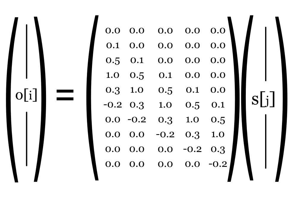
For computer simulations, there are many details to keep track of, especially issues relating to the edge and wrapping. For example, we often treat the point spread functions as ‘circular’, so when a value shifts below the bottom of the matrix, we do not throw it away but we copy it into the missing entry at the top of the column. In Figure 31.1, the edges of the point spread are all zero, and that made the diagram simpler.
Have a good look at Figure 31.1. Notice how simple an LSI system matrix is compared to a general linear system Figure 29.1. Linear systems are great to work with, and if you are working with an LSI consider yourself particularly fortunate. The next section gives another reason why.
31.3 Convolution
The matrix multiplication for a space-invariant system, which we visualized as a sum of scaled and shifted point spread functions, is often expressed using a basic formula, known as convolution.
Formally, for signals of length \(N\) with periodic boundary conditions (circular wrap), the convolution of an input signal \(I[n]\) with a point spread function \(h[n]\) is \[ O[n] = (I * h)[n] = \sum_{k=0}^{N-1} I[k]\,h[(n-k)\ \bmod\ N]. \tag{31.2}\]
Here, the output at position \(n\) is a weighted sum of the input values, where the weights are determined by a “flipped and shifted” version of the PSF. This formula is the mathematical expression of the process shown in the LSI matrix tableau.
Convolution is the essential calculation for determining the output of any LSI system in the spatial domain. With periodic boundaries this is circular convolution. To realize linear (non-wrapping) convolution in practice, zero‑pad the signals (to at least \(N+M-1\)) before transforming.
31.4 Eigenvectors of LSI Systems
We’ve arrived at a key insight: harmonic functions are a very useful basis for describing LSI systems. Why? Because they are (nearly) the eigenfunctions of these systems.
Recall that an eigenvector of a matrix is a special vector that, when multiplied by the matrix, is simply scaled—its direction doesn’t change. Harmonics play a similar role for LSI systems. When you input a harmonic function (a sine or cosine wave) into an LSI system, the output is always a harmonic of the same frequency. They aren’t quite eigenvectors because two things change: the amplitude and phase (position).
Dealing with separate amplitude and phase changes for real-valued sine and cosine functions can be a bit clumsy. This is where complex numbers become incredibly useful. A single complex number elegantly packages both amplitude (as its magnitude) and phase (as its angle). By representing our real-valued harmonics using complex exponentials (via Euler’s formula, Equation 31.8), the “almost an eigenfunction” relationship becomes exact. A complex exponential input to an LSI system produces a complex exponential output, scaled by a single complex number that captures both the amplitude and phase change.
So, we can state this powerful fact: complex exponentials are the eigenvectors of any LSI system.
This is more than a mathematical curiosity. The complex exponentials form a complete, orthogonal basis (Section 29.5). This means any image can be perfectly represented as a weighted sum of these functions, and we can efficiently transform between the point representation and the harmonic representation (Section 31.6).
I’ll admit, using complex numbers can feel strange at first. After all, our lab instruments measure real-valued signals, not imaginary ones. I often find it helpful to remember that complex exponentials are just a convenient way to handle the sine and cosine components simultaneously. They are a powerful mathematical tool, not a physical reality.1
The bottom line is that the eigenvector relationship between harmonics and LSI systems simplifies everything. Instead of tracking how every single point in an image is transformed, we only need to know how the system scales the amplitude and shifts the phase of each harmonic frequency. This simplification is the foundation of Fourier analysis in image systems.
As a young assistant professor, I had the privilege of being in faculty meetings with senior colleagues I deeply admired—Joe Goodman, Ron Bracewell, Tom Cover, and others. We often debated how to best teach core mathematical concepts to engineering students.
A recurring topic was whether to start with continuous functions and calculus or with discrete signals and linear algebra. The senior faculty, steeped in the classical tradition, generally argued for the continuous case. They saw functions and integrals as the fundamental “reality.” I vividly remember Ron Bracewell describing the discrete, matrix-based methods we use for computation as a “vulgar” but necessary approximation of this underlying truth.
The younger faculty, who spent most of our time programming, tended to favor starting with vectors and matrices. This approach felt more direct and intuitive for building computational tools.
These were spirited debates, born from a shared passion for teaching. Today, linear algebra is the language of modern computational science, from machine learning to the image systems in this book. That’s why I’ve chosen the matrix-first approach here. Still, I often think of Ron’s advice and the importance of understanding the continuous-domain theory that these discrete methods represent.
It’s also worth remembering that matrix methods are not just a modern computational fad; they have a rich history stretching back nearly two centuries. If you’re interested, you can read more about the history of these powerful ideas.
31.5 Discrete Fourier Series (DFS)
We have now arrived at the tooling we use to analyze LSIs with harmonics. The first idea is to represent image stimuli using harmonic functions. When we work with discrete, sampled data -like images- the representation is called Discrete Fourier Series (DFS). The DFS represents sampled data as sums of harmonics[^1d-simplification].
For a sampled 1D signal we write \(I[n]\) with \(n = 0,\ldots,N-1\) (there are \(N\) samples). The DFS uses integer spatial frequencies \(f = 0,\ldots,N-1\) and assumes the signal repeats every \(N\) samples (periodic extension). Here are three equivalent forms.
- Sine–cosine form
\[ I[n] = \frac{a_0}{2} + \sum_{f=1}^{N-1} \, s_f \,\sin\!\left(\frac{2 \pi f n}{N}\right) + c_f \,\cos\!\left(\frac{2 \pi f n}{N}\right) \tag{31.3}\]
- Amplitude–phase form
\[ I[n] = \frac{a_0}{2} + \sum_{f=1}^{N-1} a_f \,\sin\!\left(\frac{2 \pi f n}{N} + \phi_f\right), \qquad a_f \ge 0 \tag{31.4}\]
- Complex exponential form
\[ I[n] = \sum_{f=0}^{N-1} w_f \, e^{\,i \, 2 \pi f n / N}, \tag{31.5}\]
where the weights \(w_f\) are complex and \(i = \sqrt{-1}\).
31.6 Discrete Fourier transform (DFT)
We need a way to transform the sampled image intensities, \(I[n]\), into the Fourier weights, \(w_f\). The method is called the Discrete Fourier Transform (DFT): \[ w_f = \frac{1}{N} \sum_{n=0}^{N-1} I[n] \, e^{-i 2 \pi f n / N} \tag{31.6}\]
Because the basis is orthogonal (Section 29.6), the inverse can also be expressed directly, \[ I[n] = \sum_{f=0}^{N-1} w_f \, e^{\,i 2 \pi f n / N}. \tag{31.7}\]
At first glance, because of the use of complex exponentials, this formula might look intimidating. But take a moment, it’s actually quite simple. On the right, we have the sampled image values multiplied by a complex exponential. You might imagine this as a matrix multiplication in which we place \(I[n]\) into a vector and we place the complex exponentials into the columns of a matrix. This is the idea we explained in general terms in Section 29.5.
For some, it is preferable to get rid of the complex notation. Thanks to Euler’s formula, we know that any complex exponential can be written in terms of sine and cosine:
\[ e^{i\theta} = \cos(\theta) + i\sin(\theta). \tag{31.8}\]
This means the DFT uses the complex exponential as a method to combine the familiar sine and cosine terms into a compact expression. Once you get used to it, this complex formulation will seem neater than keeping track of separate sine and cosine coefficients.
It’s important to note that while \(I[n]\) is real-valued, the DFT coefficients \(w_f\) are generally complex. For a real signal, there is redundancy: the coefficients satisfy \(w_{f} = \overline{w_{N-f}}\), where \(\overline{w_f}\) is the complex conjugate of \(w_f\).2
If you prefer to work with real numbers, you can compute the sine and cosine coefficients, \(s_f\) and \(c_f\), directly from the image intensities:
\[ \begin{aligned} a_0 &= \frac{2}{N} \sum_{n=0}^{N-1} I[n] \\ s_f &= \frac{2}{N} \sum_{n=0}^{N-1} I[n] \sin\left(\frac{2\pi f n}{N}\right) \\ c_f &= \frac{2}{N} \sum_{n=0}^{N-1} I[n] \cos\left(\frac{2\pi f n}{N}\right) \end{aligned} \]
Here, \(a_0\) gives twice the mean value of \(I[n]\), which is why the Discrete Fourier Series (Equation 31.3) starts with \(\frac{a_0}{2}\).
31.7 Relating the DFS representations
There are several equivalent ways to write the Discrete Fourier Series, and it’s helpful to know how the parameters relate:
\(\frac{a_0}{2}\) and \(w_0\) both represent the mean value of the signal \(I[n]\).
The amplitude and phase parameters relate to the sine and cosine coefficients as follows:
\[ \begin{aligned} a_f & = \sqrt{{s_f}^2 + {c_f}^2} \\ \phi_f & = \operatorname{atan2}(c_f,\, s_f) \end{aligned} \]
Equivalently, \(s_f = a_f \cos\phi_f\) and \(c_f = a_f \sin\phi_f\). Using \(\operatorname{atan2}\) ensures the correct quadrant for \(\phi_f \in (-\pi, \pi]\).
- The complex weights \(w_f\) are related to the sine and cosine coefficients by
\[ w_f = \frac{1}{2} (c_f - i s_f ) \qquad \text{for } f > 0 \]
- And the complex weights \(w_f\) are related to the amplitude and phase by
\[ w_f = \frac{a_f}{2} e^{i (\phi_f - \pi/2)} \qquad \text{for } f > 0 \]
So, whether you prefer to think in terms of sines and cosines, amplitudes and phases, or complex exponentials, you can always translate between these forms.
See a brief biography of Fourier, who had a fascinating life. He served as a scientific adviser on Bonaparte’s Egyptian expedition and later as Prefect of Isère in Grenoble, where he pursued his theory of heat conduction and the use of trigonometric series.
In 1807 Fourier presented his heat memoir to the Paris Institute. The committee (Lagrange, Laplace, Monge, Lacroix) balked at representing arbitrary functions by trigonometric series and questioned the rigor; Biot and Poisson added objections. Fourier won the Institute’s 1811 prize, but publication lagged until 1822—evidence of the Academy’s initial resistance to what we now call Fourier series.
- Son of a tailor; Orphaned at 9
- Educated by Benedictines
- Supported the Revolution, becoming an adviser to Bonaparte in Egypt
- A statue of Fourier, erected in Grenoble, was later melted for armaments
31.7.1 Counting parameters
A length‑\(N\) real signal \(I[n]\) has \(N\) real values. The complex-valued DFS parameterization, however, seems to use more than \(N\) parameters. For example, the sine–cosine form has both \(s_f\) and \(c_f\) for each \(f\), and the complex exponential form uses \(N\) complex weights \(w_f\) (that’s \(2N\) real numbers). How can that be?
The resolution is that for real signals the Fourier coefficients obey symmetries that reduce the number of independent values back to \(N\) real degrees of freedom.
The cleanest way to see this is in the complex form. For real \(I[n]\), \[ w_{f} \;=\; \overline{w}_{\,N-f}, \qquad f=1,\ldots,N-1, \] so the coefficients come in complex‑conjugate pairs. Using Euler’s formula (Equation 31.8), these relate to the sine–cosine and amplitude–phase parameters as \[ w_f = \tfrac{1}{2}\,(c_f - i\,s_f), \qquad w_{N-f} = \tfrac{1}{2}\,(c_f + i\,s_f), \tag{31.9}\] and \[ w_f = \tfrac{a_f}{2}\,e^{\,i(\phi_f - \pi/2)}, \qquad w_{N-f} = \tfrac{a_f}{2}\,e^{\,-i(\phi_f - \pi/2)}. \tag{31.10}\]
Two special bins are purely real for real signals: - DC (\(f=0\)): only the cosine term contributes; this is the mean. - When \(N\) is even, the Nyquist bin (\(f=N/2\)): \(\sin(\pi n)=0\) for all integers \(n\), so only cosine remains. This bin is also purely real.
These symmetries remove the apparent over‑parameterization.
31.7.2 Sampling rate and Nyquist frequency
If image samples are spaced every \(\Delta x\), we say the sampling rate is \(f_s = 1/\Delta x\) (samples per unit). The Nyquist frequency is half the sampling rate, \[ f_N \;=\; \frac{f_s}{2} \;=\; \frac{1}{2\,\Delta x}, \] and is measured in cycles per unit (e.g., cycles/degree or cycles/mm for spatial signals). In DFT index units (dimensionless bin indices), \(f_N\) aligns with the bin at index \(N/2\) when \(N\) is even; when \(N\) is odd there is no bin exactly at \(f_N\).
As we saw in the previous section, because of conjugate symmetry, only about “half” of the spectrum is unique:
Even \(N\): There are two special, real bins—DC (\(f=0\)) and Nyquist (\(f=N/2\)). The remaining bins form conjugate pairs \((f,\,N-f)\) for \(f=1,\ldots,N/2-1\). The count of distinct frequency bins is \[ 1 \text{ (DC)} \;+\; (N/2-1) \text{ pairs} \;+\; 1 \text{ (Nyquist)} \;=\; N/2 + 1. \] Each conjugate pair contributes two real degrees of freedom (real and imaginary parts), and the two special bins contribute one each, totaling \(N\) real degrees of freedom.
Odd \(N\): There is no Nyquist bin. We have DC (\(f=0\)) plus conjugate pairs \((f,\,N-f)\) for \(f=1,\ldots,(N-1)/2\). The count of distinct bins is \[ 1 \text{ (DC)} \;+\; (N-1)/2 \text{ pairs} \;=\; (N+1)/2, \] again yielding \(N\) real degrees of freedom.
It is common to compute and report only this non‑redundant “half‑spectrum” (plus DC, and the Nyquist bin when \(N\) is even). In continuous‑domain sampling language, frequencies above the Nyquist frequency \(f_N\) “fold” or alias back; in DFT index terms, information in bins above \(N/2\) is redundant with bins below \(N/2\) for real‑valued signals. Some authors therefore call the Nyquist frequency the folding frequency.
31.8 The Convolution Theorem
The fact that harmonics are eigenvectors of linear, space-invariant (LSI) systems leads to one of the most powerful results in signal processing: the Convolution Theorem.
In the spatial domain, calculating the output of an LSI system requires performing a convolution—summing the input signal with shifted and scaled versions of the point spread function (PSF). This operation can be computationally intensive.
The Convolution Theorem provides an elegant and highly efficient alternative. It states that convolution in the spatial domain is equivalent to simple multiplication in the frequency domain.
Let’s formalize this. If the output image \(O[n]\) is the convolution of the input image \(I[n]\) and the system’s point spread function \(h[n]\): \[ O[n] = (I * h)[n], \tag{31.11}\]
then in the Fourier Transform domain the relationship is \[ \mathscr{F}\{O\} = \mathscr{F}\{I\} \cdot \mathscr{F}\{h\} \]
where \(\mathscr{F}\) is the Discrete Fourier Transform.
Using the complex weights notation, where \(W_f\) are the DFT coefficients of the input and \(H_f\) are the DFT coefficients of the PSF, the output coefficients \(Y_f\) are simply:
\[ Y_f = W_f \cdot H_f \tag{31.12}\]
This is a profound simplification. A complex convolution is replaced by straightforward, element-wise multiplication3. The term \(H_f\), the DFT of the point spread function, is so important that it has its own name: the Optical Transfer Function (OTF). The OTF describes how the system scales the amplitude and shifts the phase of each input harmonic.
This theorem is the primary reason why Fourier analysis is indispensable for image systems engineering. It allows us to:
- Analyze a system’s performance by examining its OTF.
- Calculate the output of an LSI system efficiently: transform the input to the frequency domain, multiply by the OTF, and transform back.
- Design systems by specifying a desired OTF.
You will see all of these ideas used in various ways in the main chapters of this book. Fourier series play a role in modeling optics and characterizing optics, modeling sensors, and analyzing perceived image quality. The harmonic basis is used as a tool in most aspects of science and engineering.
I also explain the relationship between harmonics and space-invariant linear systems in detail, staying away from complex exponentials, in the Appendix to Foundations of Vision.↩︎
The complex conjugate of \(a + i b\) is \(a - i b\).↩︎
Multiplication in the DFT domain corresponds to circular convolution in the spatial domain. To implement linear convolution without wrap‑around, zero‑pad the inputs before applying the DFT.↩︎