11 Spatial domain
The book is still taking shape, and your feedback is an important part of the process. Suggestions of all kinds are welcome—whether it’s fixing small errors, raising bigger questions, or offering new perspectives. I’ll do my best to respond, but please keep in mind that the text will continue to change significantly over the next two years.
You can share comments through GitHub Issues.
Feel free to open a new issue or join an existing discussion. To make feedback easier to address, please point to the section you have in mind—by section number or a short snippet of text. Adding a label characterizing your issue would also be helpful.
Last updated: November 6, 2025
11.1 Spatial domain
Geometric optics helps us understand how lenses work by focusing on properties like the lens shape, its material, and its distance from the sensor. This approach is excellent for designing lenses and determining their basic characteristics.
An alternative way to analyze optical systems is to treat them as signal processors. In this framework, an optical system takes light from a scene as its input and transforms it into an image at the sensor, which is the output. This signal processing perspective is powerful because it allows us to focus on what the system does—its transformation—without getting lost in the physical details of its construction. It is a practical approach for developing image system simulations and analyzing optical performance.
This method is particularly effective because many optical systems are approximately linear, meaning they satisfy the Principle of Superposition. This property can be tested experimentally. A rich set of mathematical tools exists for analyzing linear systems, taught widely across science, technology, engineering, and mathematics.
Because many readers will be familiar with linear systems, I have placed a general introduction to these concepts in Part VII: Appendix (Section 29.1). If you are already comfortable with linear systems principles, you can use that appendix to align with the notation and methods used in this book. If these ideas are new to you, I hope you will find the appendix a useful resource.
11.2 Linearity
11.2.1 Point spread functions
In Section 7.8 I introduced the idea of the point spread function (PSF). It is simply the image of a point of light. If we know the point spread for each location in the scene, and superposition holds, we can predict how any input scene becomes an image.
The scene is a collection of scene points, \(\mathbf{p} = (p_x, p_y, p_z)\), each with its own intensity \(S(\mathbf{p})\). Write the point spread function of a scene point as \(\text{PSF}_{\mathbf{p}(x, y)}\), where \((x, y)\) are positions in the image. Using superposition, we calculate the output image, \(O(x,y)\) by adding up the weighted point spreads from every scene point. The formula looks like this:
\[ O(x, y) = \sum_{\mathbf{p}} s(\mathbf{p})\, \text{PSF}_{\mathbf{p}}(x, y) \tag{11.1}\]
Here, \(O(x, y)\) is the intensity at each image position. Each point in the scene contributes a scaled version of its PSF. The output image is the weighted sum of all those PSFs.
Point spread functions are an intuitive way to understand the performance of the optical system, and they are widely used in applications. In Section 11.5 I will describe how scientists and engineers design optics to achieve specific PSF characteristics to estimate depth or to reveal hard-to-see objects.
In the Section 29.1 I describe how the point spread function is used to create the linear system matrix: each column of the linear system matrix is a point spread. When the system is space-invariant (Section 31.1), the columns of the matrix are shifted copies of that point spread. We also explain that harmonics are eigenvectors of such matrices. This section further explores the analysis of optics using PSFs, and Section 12.2 explores applications using harmonics.
Point spread functions (PSFs) are an excellent tool for modeling optical systems when the scene can be approximated as a flat surface, or when all objects are far enough away that occlusion is negligible. In these cases, each point in the scene contributes independently to the image, and the total image can be predicted by summing the PSFs from each point.
However, in three-dimensional scenes where objects can block light from those behind them (occlusion), the situation becomes more complex. The contribution of a point to the image may be partially or completely blocked by closer objects. As a result, the effective point spread depends on the arrangement of objects in the scene, and cannot be characterized by a single, scene-independent PSF. Accurately modeling these effects requires more advanced techniques, such as those used in computer graphics, and often involves recalculating the image formation for each specific scene.
In summary, PSFs provide a powerful and practical framework for image prediction when occlusion can be ignored, but their direct application is limited in scenes with significant three-dimensional structure and occlusion. In those cases, computer graphics techniques based on ray tracing are more appropriate.
11.2.2 General linear analysis
There is no guarantee that the point spread is the same everywhere in the image, and in general it will not be. This case is called a shift-varying linear system, and we represent the linear system by a general matrix (Section 29.4). In that case each column of the matrix represents the point spread for a different point. These can be quite broad and irregular, making the image quite unrecognizable. Even so, if we know the matrix, and it is invertible, we can estimate the input.
The calculation is illustrated in the script fise_ImageFormationLinearity. I created a random image to serve as the PSF for each pixel, and naturally the image looks completely random. But with knowlege of the PSFs, and thus the system matrix, we can find the inverse of the system matrix and estimate the input from an image that appears to be complete noise.
There are many details as to how well this works, mostly concerning how robust the calculation is to noise. I doubt this calculation is of practical interest, though it has been used in interesting ways by Laura Waller’s group. (Correct me if you know of a case!) The principle of linearity is good to keep in mind because it will help you solve many other problems.
11.2.3 Space invariant linear analysis
A more common situation for image systems engineering is the shift-invariance: the point spread is the same over a some region (isoplanatic region). We have many powerful mathematical tools for simulating and analyzing this case (Chapter 31). This is the case in which we can compute the system transformation using convolution (Section 31.3) and Fourier tools (Section 31.8).
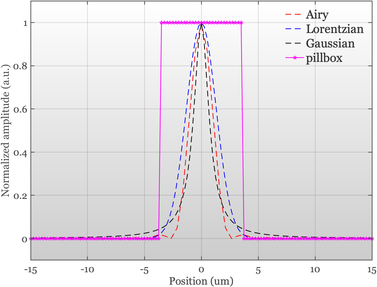
11.3 Common PSFs in simulation
The PSFs of real systems can be difficult to model using a simple formula. In ISETCam we make it possible to provide an empirical PSF when it is known. But there are many cases in which the PSF is not yet known, say for a system that is under design and the optics have not yet been selected. In such optical system simulations, a few PSFs are routinely used to approximate image system performance prior to implementation (Figure 11.1).
- Airy pattern is the only one of these PSFs that is based on the physics of light waves. This is the PSF we measure for a perfect, diffraction-limited lens imaging a point at a distance (Section 7.7 and Figure 7.12). The Airy pattern depends on wavelength and represents a best case limit. The optics you use will not be better than this.
- Gaussian is popular because it’s easy to work with in calculations.
- Lorentzian (also called Cauchy) has higher tails than the Gaussian. This makes it better for modeling systems where light gets scattered a lot—like if the lens is scratched or there are many internal reflections from a multi-element lens assembly.
- Pillbox A square region with constant values that averages the values over the region. Who doesn’t like a simple average? Well, I don’t - but apart from me?
A graph of the cross-section through these PSFs is a useful way to compare them.
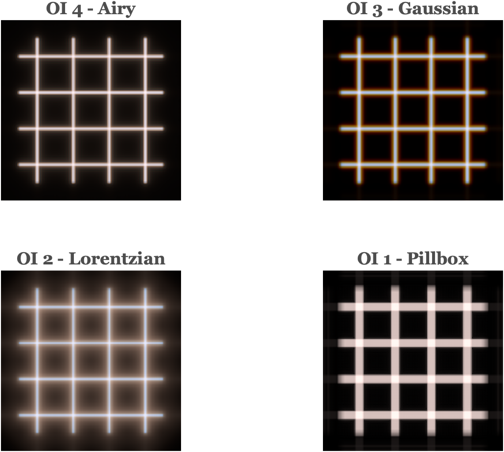
We can simulate how the four PSF shapes transform a spectral radiance (Figure 11.2). We compare the optical images four each of the PSFs for a scene comprising a set of grid lines. The images were calculated using the ISETCam script fise_opticsPSF. The Airy and Gaussian PSFs were implemented with wavelength-dependent point spread functions. The Pillbox and Lorentzian PSFs were implemented as wavelength-indepedent.
These PSFs are valuable because they have simple parameters that control the amount of blur or light scatter. Here is a description of the different PSF formulae along with a brief descrition of their properties.
11.3.1 The Airy pattern
The Airy pattern is circularly symmetric, so you only need to know the distance from the center, \(r\), to describe it. The intensity at a distance \(r\) from the center is:
\[ I(r) = I_0 \left[ \frac{2 J_1\left( \frac{\pi r}{\lambda N} \right)}{ \frac{\pi r}{\lambda N} } \right]^2 \]
Where:
- \(I_0\) is the peak intensity at the center
- \(J_1\) is the first-order Bessel function
- \(N\) is the \(f/\#\) of the lens
- \(\lambda\) is the wavelength of light
The first dark ring defines the Airy disk (Figure 7.12 , Section 7.7). It is the diameter where the intensity drops to zero, and defines the smallest spot size.
\[ d = \arcsin(2.44 \, \lambda N) \approx 2.44 \, \lambda N \tag{11.2}\]
For \(f/\# = 4\) the diameter ranges from 3.9 \(\mu\text{m}\) (400 nm) to 6.83 \(\mu\text{m}\) (700nm). See the ISETCam function airyDisk
11.3.2 Gaussian
The Gaussian is the classic “bell curve.” It’s simple and often a used as an approximation for optical systems. \[ I(r) = I_0 \exp\left( -\frac{r^2}{2\sigma^2} \right) \]
Here, \(\sigma\) sets how spread out the blur is. Larger \(\sigma\) means a blurrier image.
11.3.3 Lorentzian (Cauchy)
The Lorentzian function appears in physics and probability theory. It’s famous for its “fat tails”—meaning it doesn’t drop off as quickly as a Gaussian. This makes it handy for modeling blur when there’s a lot of stray light or scattering.
\[ I(r) = \frac{I_0}{1 + \left( \frac{r}{\gamma} \right)^2} \]
Here, \(\gamma\) controls how wide the central peak is. A bigger \(\gamma\) means a wider, flatter blur with more light in the tails.
All of these PSFs are simulated in siSynthetic.m.
The impact of different point spreads can be easier to measure and visualize using line inputs rather than points. The image created by a very thin line is called the line spread function (LSF).
To find the LSF from the PSF, we simply sum along the direction (psf2lsf.m). The LSF is the same in any direction when the PSF is cicularly symmetric. Otherwise, the LSF differs with direction.
The formula to calculate the PSF in a direction, in this case the \(y\) direction, is very simple. We just sum across the \(x\) direction.
\[ LSF = \sum_x PSF(x,y) \]
Here are the linespread functions of the Gaussian and Lorenzian.
Given an LSF, it is possible to recover a unique circularly symmetric PSF using lsf2circularpsf.m. The Airy pattern is circularly symmetric; the Gaussian and Lorentz are usually implemented as circularly symmetric. The pillbox is not.
One of the challenges in image system simulations is to select the wavelength dependence of the PSF. This dependence is formally specified for the Airy pattern, based on the wavelength of light and the size of the circular, pinhole aperture. But for the Gaussian and Lorentzian, we must make a choice.
One way to make a decision is to measure the wavelength dependence for an existing system, say a system that uses materials with known properties, and use those measurements to guide the simulation. The variations in the PSF caused by these wavelength-dependences are called chromatic aberrations. There are two types of chromatic aberrations, and we describe them and how they might be measured in the next section.
11.4 Accounting for wavelength
Because the index of refraction of a lens might vary with wavelength, the best focus distance also varies with wavelength (Section 8.3.2). Even for an ideal lens there is a wavelength dependence arising from the wave nature of light and the size of the aperture or \(\text{f}/\#\) (Equation 7.1).
11.4.1 Longitudinal chromatic aberration
A consequence of this wavelength-dependence is that for a given image distance will be in best focus (small PSF) for one wavelength, but not all. The wavelength-dependent defocus is called longitudinal chromatic aberration (LCA).
There is noticeable chromatic aberration for many types of lenses and materials. The most surprising optical system with a large amount of chromatic aberration is the human eye! The line spread and point spread functions measured at the human retina both vary considerably as we change the stimulus wavelength.
The very large LCA of the human eye has consequences for many aspects of the human visual system and image systems engineering technology. We will describe it quantitatively and explain why it matters to technology in Section 23.1.
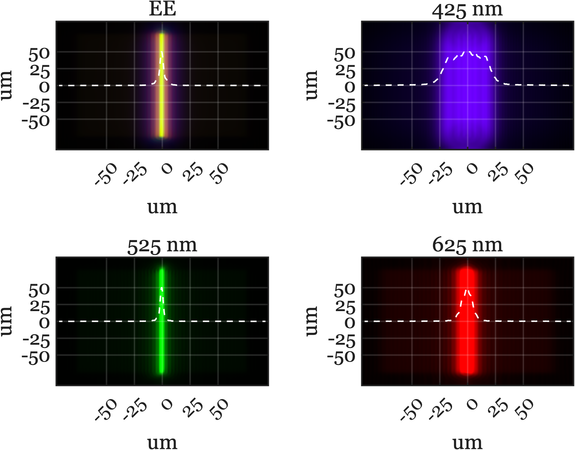
11.4.2 Transverse chromatic aberration
A second type of chromatic aberration, called transverse chromatic aberration (TCA), is also common in real imaging systems. While it is related to LCA, its physical cause is different.
TCA occurs when the image blur interacts with the position and size of the aperture. The two panels of the figure below show short wavelength (blue) and long wavelength (red) rays, originating from a point at the lower left. The blue rays are in focus, forming a tight spot on the image plane. The red rays, however, come to focus behind the image plane, creating a larger, blurred red circle.
Now, imagine reducing the aperture size and moving it in front of the lens. This new aperture position blocks some of the rays from both wavelengths. For the blue rays, which were already converging to a tight focus, the effect is minimal —the spot gets a little dimmer. But for the red rays, which form a large blur circle already, the new aperture blocks rays that would have formed the lower part of their blur circle. As a result, the red blur circle is clipped at the bottom, and its center shifts upward. The red and blue circles are no longer aligned. The displacement of the red blur circle is transverse chromatic aberration.
The size and position of the aperture determines the amount of TCA. The physical factors that cause the transverse shift are different from those that produce LCA. Both effects are related to the different wavelengths focus. Were there no LCA, there would be no TCA.
11.5 PSF engineering
The usual goal of optical design for consumer photography is to create a lens that has a very compact point spread function (sharp image) that is the same for all wavelengths (no chromatic aberration). This makes sense because people want their photographs to be sharp and free of the kind of chromatic fringing you can see in Figure 11.3 (a) and Figure 11.3 (b).
The goal of optical design can differ, of course, for different applications. In the sections below, I describe two cases that I found to be very interesting. The first case designs optics for telescopes that are looking for planets in other star systems (exoplanets). The second case designs optics that can be helpful in estimating the depth of objects in an image. For example, in microscopy we might be interested to measure the tissue layer where a particular glowing molecule resides. These two examples are drawn from the literature of PSF engineering.
11.5.1 Exoplanets
When we see a solar eclipse, the moon blocks the bright center of the sun, revealing the faint outer atmosphere called the corona. For centuries, scientists could only study the corona during these rare events. That changed in the 1930s, when Bernard Lyot invented the coronagraph—an optical instrument designed to block out the sun’s bright disk and make the corona visible at any time.
The key to a coronagraph is PSF engineering: designing the optics so that light from a bright central source (like the sun or a star) is strongly suppressed in the image. By shaping the point spread function (PSF) to have a dark center, the instrument allows much fainter features near the bright source to be detected. Lyot’s original design remains influential and is still used in modern telescopes, including the James Webb Space Telescope’s coronagraphic instruments. The basic layout is shown in Figure 11.5. 1
Here’s how the Lyot coronagraph works (Figure 11.5): Parallel rays from a distant star or the sun enter the telescope and are focused by the first lens. At the focal plane, a small opaque disk (the occulting disk) blocks the bright central spot. This also introduces some diffraction, as light bends around the edge of the disk. A second lens then reimages the entrance pupil, creating a new pupil plane. In this plane, a Lyot stop—a slightly smaller aperture—blocks much of the diffracted light. Finally, a third lens forms the final image, where the bright core is suppressed and the faint corona or nearby objects become visible. Typically, only about 1/200th of the original light makes it through the system.
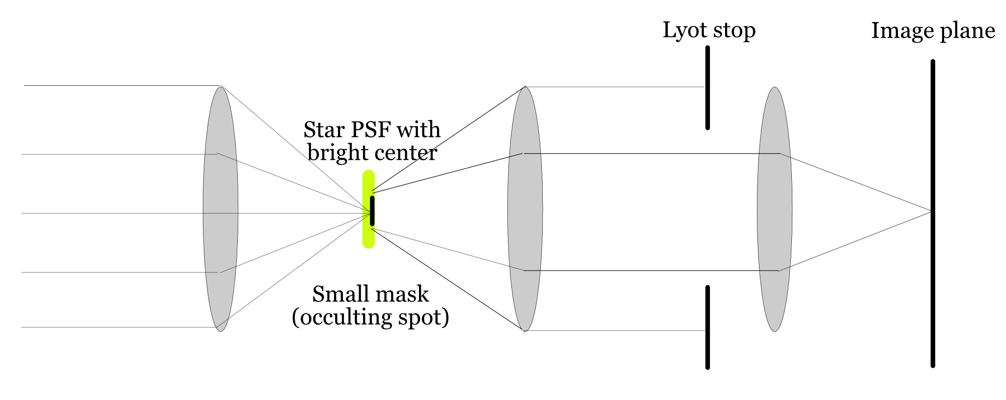
Modern coronagraphs go beyond simple stops. They use specially shaped apertures and optical elements that adjust the phase of the incoming light, creating a PSF with an extremely dark center. One way to design the Lyot stop is to determine the diffraction pattern expected from the occulting stop and then use a Lyot stop that blocks the locations where the diffracted light is most intense.
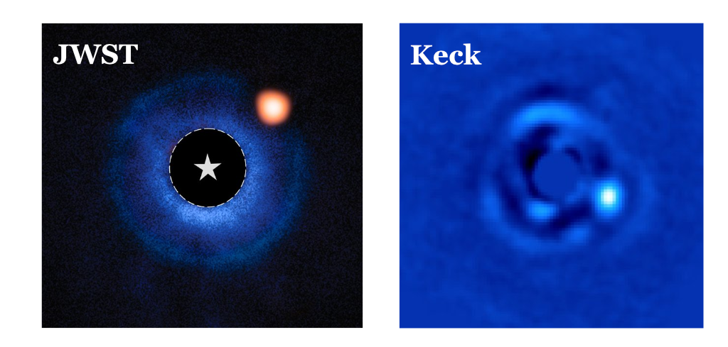
The PSF engineering first developed for coronagraphs is crucial for direct imaging of exoplanets, which are the planets orbiting other stars. The challenge is to block the overwhelming starlight so that the faint reflected light from a nearby planet can be detected. One ambitious project, the Exo-Life Finder (ELF), uses advanced coronagraphic PSF engineering to search for signs of life on exoplanets (Kuhn et al. (2025)):
The telescope we’d like to design and build targets the problem of finding life around planets outside the solar system. To do this requires separating the reflected starlight off the planet from the star. Astronomers call this “direct imaging.” This means we’re interested in optical systems that can have a narrow field-of-view (FOV), perhaps just a few arcseconds, and enormous photometric dynamic range capability. A laudable goal is to achieve raw sensitivity of \(10^{-8}\) of the stellar flux in a region within about 1 arcsecond of the central star. A dedicated telescope with this capability could make images of the surface of nearby exoplanets using data inversion techniques, perhaps sufficient to see even signs of advanced exolife civilizations (Kuhn et al. (2025)).
In very modern designs the simple stops are replaced by optical components that control the phase of the light across the pupil (Kuhn et al. (2025)). This additional control creates a PSF with a central region that is suppressed by eight orders of magnitude or more—an essential requirement for exoplanet imaging. Achieving this level of control in a large instrument is a major technical challenge, involving not just optics, but also mechanical engineering, materials science, signal processing, and even project management and funding.
The search for exoplanets is a striking example of how PSF engineering can be used to push the limits of what we can observe, revealing new worlds that would otherwise remain hidden in the glare of their parent stars.
11.5.2 Microscopy and depth
A second excellent application of PSF engineering is found in microscopy, where it is used to determine the three-dimensional position of molecules within biological samples. Biologists often use fluorescent markers to tag specific molecules in tissue. When excited by light of one wavelength, these tags emit light at another, making them visible under a microscope. A single fluorescent molecule is so small that it acts as a point source, and its image through the microscope is a PSF.
This principle is the foundation for a set of techniques known as Single Molecule Localization Microscopy (SMLM). The origins of SMLM trace back to the work of W.E. Moerner, who first demonstrated that it was possible to detect light from a single fluorescent molecule and that these molecules could be switched on and off with light (Moerner and Kador (1989), Dickson et al. (1997)).
Building on this, researchers like Eric Betzig (Photoactivated Localization Microscopy, PALM) and Xiaowei Zhuang (Stochastic Optical Reconstruction Microscopy, STORM) developed methods to create images with unprecedented detail (Betzig et al. (2006), Rust et al. (2006)). The key idea is to activate only a sparse subset of fluorescent tags at any given moment. Because the active molecules are far apart, their PSFs do not overlap. The center of each PSF can be calculated with high precision, revealing the molecule’s \((x, y)\) position. By repeating this process—activating a new sparse set of molecules, localizing them, and then combining all the locations—a complete, high-resolution image is constructed.
These SMLM techniques are often said to “break the diffraction limit” because they can localize molecules on a scale much smaller than the Airy disk. This has revolutionized biological imaging, earning Moerner, Betzig, and Stefan Hell2 a Nobel Prize.
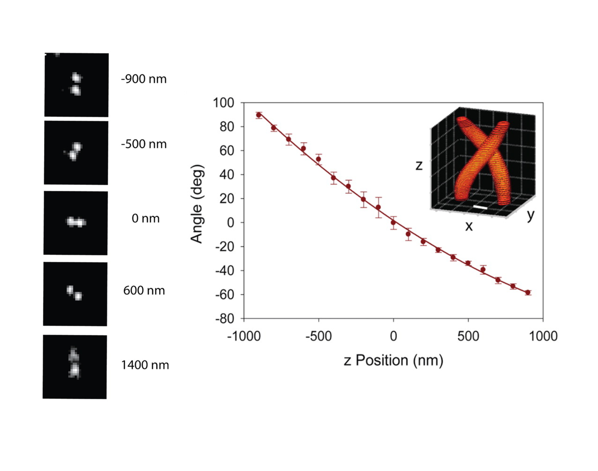
While SMLM excels at finding the \((x, y)\) position, determining a molecule’s depth (\(z\) position) is also critical for understanding 3D biological structures. The PSF of a conventional microscope changes with depth, but usually just by becoming slightly more blurry, which is difficult to measure accurately.
This is where PSF engineering provides a brilliant solution. Rafael Piestun and his collaborators designed an optical system that transforms the PSF into a distinctive shape: two lobes that rotate around a central point as the molecule’s depth changes (Pavani and Piestun (2008)). When plotted as a function of depth, the rotating lobes trace out a double helix (Figure 11.8). For a sparsely labeled sample, an investigator can find the \((x, y)\) position from the PSF’s center and estimate the depth (\(z\)) from the orientation of the two lobes. This clever design enables precise 3D localization of single molecules. Piestun co-founded Double Helix Optics to commercialize this technology.
The image formation in a coronagraph involves a sequence of Fourier Transforms between pupil and image planes. This mathematical framework allows us to predict how well the system will suppress unwanted light. We’ll explore these calculations in later sections. ↩︎
Stefan Hell developed a different but related super-resolution approach called STED microscopy. It uses a special pattern of light to shrink the region where fluorescence occurs, also achieving very high spatial resolution.↩︎