12 Transform domain
The book is still taking shape, and your feedback is an important part of the process. Suggestions of all kinds are welcome—whether it’s fixing small errors, raising bigger questions, or offering new perspectives. I’ll do my best to respond, but please keep in mind that the text will continue to change significantly over the next two years.
You can share comments through GitHub Issues.
Feel free to open a new issue or join an existing discussion. To make feedback easier to address, please point to the section you have in mind—by section number or a short snippet of text. Adding a label characterizing your issue would also be helpful.
Last updated: November 22, 2025
12.1 Transform domain overview
We have mainly been analyzing optical systems using point-based stimuli (impulses and point spread functions). This is one of many useful signal representations (Chapter 29). In this section, we introduce a second class of stimuli: image harmonics. These stimuli are commonly used in the image systems engineering literature for both theory and measurement. They provide a valuable and insightful approach to measuring how image systems behave.
There are two practical motivations for considering alternative stimuli. First, point stimuli are not convenient tools for predicting how finely a system can resolve detail; the spatial resolution of an image system is often easier to analyze using harmonics. Second, point stimuli are photon-inefficient and thus difficult to measure precisely. Extended harmonic targets deliver more light, produce higher signal-to-noise measurements, and allow precise control of spatial frequency, orientation, and phase.
The next sections define image harmonics and show how to use them to characterize system performance. The mathematical foundations underpinning this representation appear in Chapter 29 and Chapter 30. In brief: for linear, space-invariant systems, harmonics form a spatial basis for arbitrary stimuli (Section 29.5) and are nearly eigenfunctions of the system (Section 29.7). These properties make harmonics especially valuable for analysis and design.
12.2 Image harmonics
For real-valued signals —such as light intensity— the harmonics are built upon the sine and cosine functions. You likely first met these as one-dimensional functions: they take a single input and produce a single output that varies from \([-1,1]\).
\[ I(x) = \sin(2\pi f_x x + \phi_x) \tag{12.1}\]
Here, \(f_x\) is the spatial frequency (in cycles per unit distance) and \(\phi_x\) is the phase (a spatial shift). Image intensities are positive numbers, so to model them with harmonics we add \(1\) to the value.
\[ I(x) = 1 + \sin(2\pi f_x x + \phi_x) \tag{12.2}\]
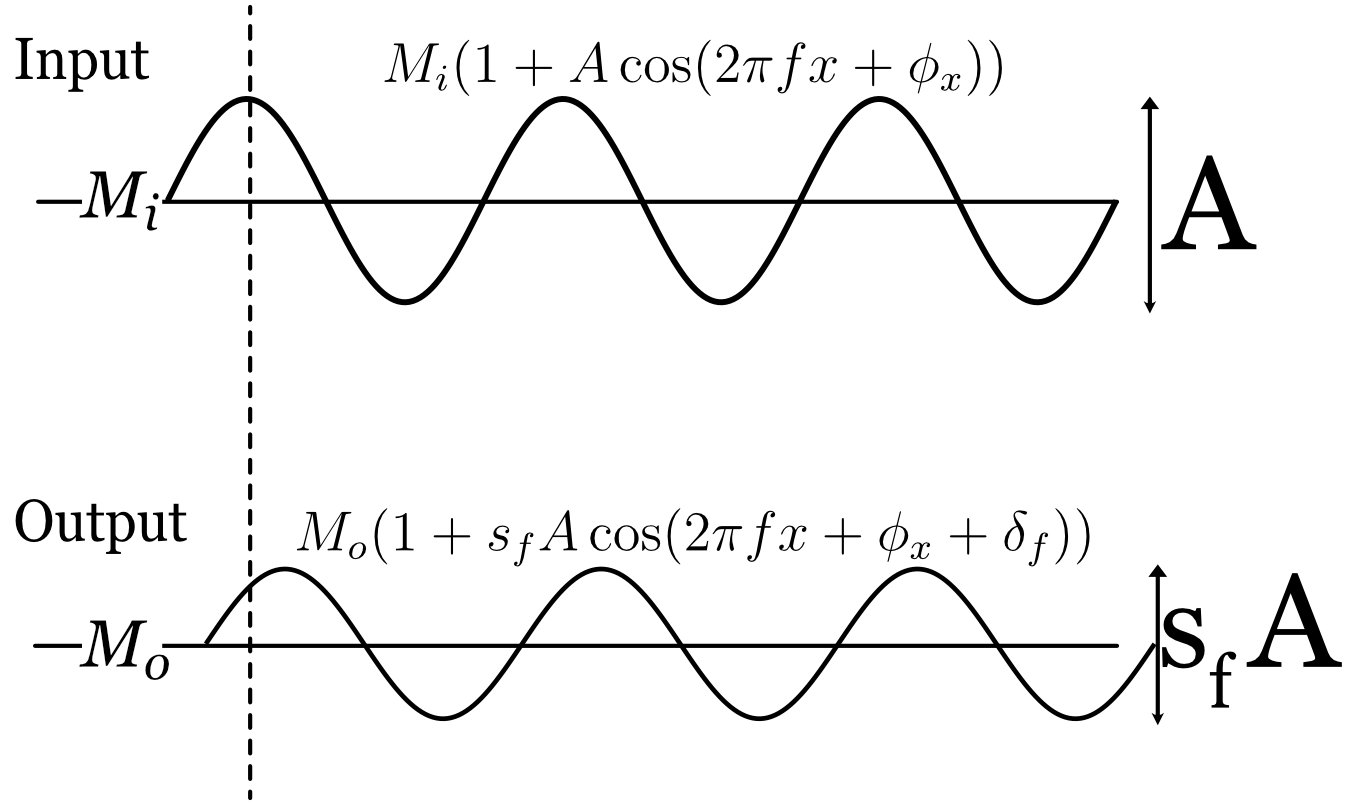
In imaging, we typically need a two-dimensional representation to describe variation across both \(x\) and \(y\). A compact form that keeps intensities non-negative is \[ I(x,y) = M\big(1 + A \,\sin\big(2\pi (f_x x + f_y y) + \phi\big)\big). \tag{12.3}\]
- \(M\) is the mean (DC) intensity.
- \(A\) is the contrast or modulation depth. To ensure \(I(x,y)\ge0\), require \(|A|\le 1\) (in practice, take \(A\in[0,1]\) and absorb the sign into \(\phi\)).
- \((f_x,f_y)\) defines the 2D spatial frequency. The orientation is \(\theta=\mathrm{atan2}(f_y,f_x)\) and the radial frequency is \(\| \mathbf{f} \| = \sqrt{f_x^2+f_y^2}\).
Figure 12.1 shows four image harmonics. When \(f_y = 0\) the pattern is vertical (varies only along \(x\)); when \(f_x = 0\) it is horizontal (varies only along \(y\)).1

For many linear-systems analyses, say when the system is circularly symmetric, it is enough to consider one-dimensional harmonics by fixing \(f_y = 0\). The examples in Figure 12.2 vary only along \(x\) and illustrate different spatial frequencies \(f_x\) and contrasts \(A\).

To many people it is counterintuitive that a thin line can be constructed by summing harmonics. The line is very compact, but each harmonic extends across the entire image. How can the sum of these harmonics functions result in such a localized image?
Figure 12.3 shows how the image evolves as we sum increasing numbers of harmonics: Starting with just a few, the result is broad and diffuse, but as more harmonics are added, the image becomes increasingly concentrated. The key is that the positive and negative regions of the higher frequency harmonics cancel each other out everywhere except at the center, where all the cosine terms are positive (\(\cos(0)\)). With enough harmonics, the sum converges to a single, sharp line.
In this example, we reconstruct a line at the center (column 65) of a 129-column image by setting all harmonic weights to \(w_f = 1\). Because the target image is even symmetric, only the cosine terms are needed. The red traces in the figure show the intensity profile: as more harmonics are added, the central peak narrows and side ripples diminish. By the \(64^{th}\) harmonic, the line is well-formed; adding more harmonics briefly reintroduces some ringing, which disappears when the full set is included. This phenomenon is a classic result in linear systems—ask your instructor for more details!
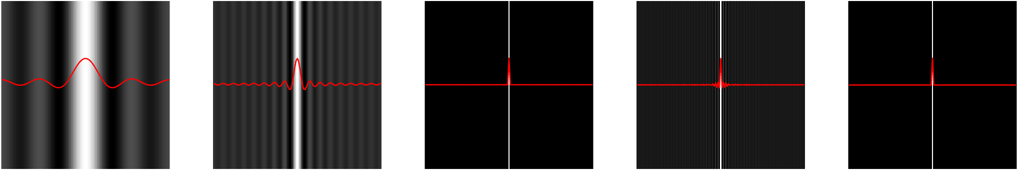
This movie illustrates how the sum converges as harmonics are added one by one. Initially, the harmonics are distributed across the image. As more are included, their contributions cancel everywhere except at the central position (\(0\)), where all are positive (\(\cos(0)\)).
Adding harmonics from \(f=0\) to \(f=64\) produces the line; adding \(f=65\) to \(f=128\) introduces some ringing, which is eliminated when the sum is complete. This is a special case for even symmetric functions, where only cosines are required.
12.3 Harmonic characterization
There are many reasons why people would like to describe the quality of an optical system. Commercial vendors that sell parts may need to specify the quality and the tolerance of the quality measure. We may want to optimize the properties of a design, using the image quality measure as a metric for the optimization. We may wish to simulate the system and learn which signals are preserved by the optics and which are lost to image quality.
The point spread function characterizes the system using many values measured from a single stimulus. The harmonic characterization uses only two parameters, but from multiple stimuli (Figure 12.5). For each harmonic frequency, we measure how much its amplitude is scaled, \(s(\mathbf{f})\), and how much the image has been shifted \(\phi(\mathbf{f})\).
12.4 Transfer Functions
For a linear, space-invariant system, the effect of the optics on any harmonic stimulus is simple: the output is also a harmonic of the same frequency, but its amplitude is scaled and its phase is shifted. There is a small collection of transfer functions that serve as useful, compact mathematical descriptions of this scaling and shifting across all spatial frequencies. These transfer functions in the transform domain are all related to the functions in the space domain through the convolution theorem.
From Section 31.8 we have for an input, \(i\), a point spread \(h\), and an output, \(g\), the convolution represents the LSI transformation \[ g(x) = h(x) * i (x) \]
and the transform domain this is \[ \mathscr{F}(g) = \mathscr{F}(h) \cdot \mathscr{F}(i) \]
12.4.1 Optical Transfer Function
The optical transfer function (OTF), \(\mathcal{O}(f)\), is defined as the Fourier transform of the output divided by the Fourier transform of the input. From its definition, it is also the Fourier transform of the point spread function. \[ \mathcal{O}(f) = \frac{\mathscr{F}\{g\}}{\mathscr{F}\{i\}} = \mathscr{F}\{h\}. \tag{12.4}\]
The OTF is a complex function of spatial frequency. It can be written in magnitude–phase form as \[ \mathcal{O}(f) = \mathcal{M}(f)\, e^{\,i\,\mathcal{P}(f)}, \tag{12.5}\]
The term \(\mathcal{M}(f)\) is the real-valued amplitude scaling factor, and \(\mathcal{P}(f)\) is the phase shift (in radians).
The OTF provides a powerful way to predict the system’s output. Using the convolution theorem (Section 31.8), we can calculate the output image, \(g(x,y)\), by multiplying the Fourier transform of the input image, \(i(x,y)\), with the OTF and then taking the inverse Fourier transform: \[ g(x) = \mathscr{F}^{-1}\!\big( \mathcal{O}(f)\,\mathscr{F}\{i\} \big). \tag{12.6}\]
Just like its partner in the space domain, the point spread function, the OTF completely characterizes a linear, space-invariant system.
12.4.2 Modulation Transfer Function
Many times we are primarily interested in how the system affects the contrast (or modulation) of the input harmonics, without regard to the phase shift. This is captured by the modulation transfer function (MTF): \[ \mathcal{M}(f) = |\mathcal{O}(f)|. \tag{12.7}\]
For many optical systems, particularly those with symmetric point spread functions, the phase shifts are small (i.e., \(\mathcal{P}(f)\approx 0\)), in which case the OTF is approximately real and non‑negative.
Figure 12.6 illustrates the effect of the MTF. An input image with a sweep of spatial frequencies (top) is passed through an optical system. The output image (bottom) shows that the contrast of the high-frequency patterns is significantly reduced, a direct visualization of the MTF’s attenuation of higher frequencies.
https://ethw.org/Otto_H._Schade
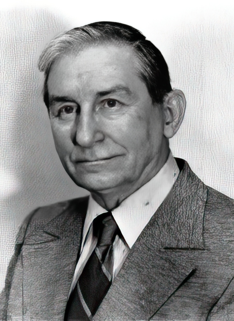
Otto H. Schade (1903–1981), an RCA engineer, is the single most important figure in bringing modulation transfer function (MTF) and linear-systems analysis into practical image-system engineering. In 1938 he began specialized studies of television circuits, camera tubes, picture tubes, and the analysis of television systems performance. From 1944 to 1957 he worked on a unified general method of image analysis and specification, including practical methods for measuring the modulation transfer function and noise in optical, photographic, and electronic imaging systems. His contributions include:
- Introducing MTF as the central system-level metric for image quality in photography, television, and film.
- Showing how lenses, film, detectors, display phosphors, and even human vision could be treated as cascaded linear filters.
- Publishing a series of influential papers from the late 1930s through the 1950s, especially the canonical 1948–1958 RCA technical reports.
- Establishing the idea that image quality is best characterized in the frequency domain, rather than by geometric aberrations alone.
In the August 1976 Scientific American, William H. Price of Kodak wrote: ” Much of the mystery surrounding lens ‘quality’ was cleared up in 1951 when Otto H. Schade, Sr., of the Radio Corporation of America, described his investigation of lenses used in the entire chain of information transmission represented by a television system.” He adds that with Otto Schade’s concepts and a computer, ” [now] we can mathematically model the entire photographic system, beginning with the subject and ending with the transfer function of the viewer’s eye Source: NAE.“. The application to the human visual system was really quite remarkable, and I will explain this in much more detail in Section 22.1.
12.4.3 Phase Transfer Function
The phase shift (in radians) as a function of frequency is called the phase transfer function (PTF): \[ \mathcal{P}(f) = \phi(f). \tag{12.8}\]
Putting these terms together, we have simply
\[ \mathcal{O}(f) = \mathcal{M}(f) \, e^{\,i \, \mathcal{P}(f)} . \tag{12.9}\]
12.4.4 Contrast Sensitivity Function
For some systems, we cannot directly measure the output signal. The human visual system is a prime example: we can ask a person what they see, but we cannot easily measure the neural response at the retina or in the cortex. This “black box” problem is common in many fields.
A clever way to characterize such systems is to measure the input required to produce a constant, predefined output. This general approach is known by various names: “input-referred measurement” in engineering, “action spectrum” in photobiology, and “Type A” experiments in physiology (Brindley (1970)).
In vision science, this method is used to define the contrast sensitivity function (CSF), \(\mathscr{C}(f)\). To measure the CSF, an observer is shown a harmonic pattern of a specific frequency, and the contrast is adjusted until the pattern is just barely visible (at the detection threshold). This process is repeated for many different spatial frequencies.
The contrast sensitivity for a given frequency, \(f\), is defined as the reciprocal of the threshold contrast, \(A_{f}\):
\[ \mathscr{C}(f) = \frac{1}{A_{f}} \]
For example, if a spatial frequency pattern at \(f\) is detectable at 1% contrast (\(A_f=0.01\)), the contrast sensitivity is \(1/0.01 = 100\). If a high-frequency pattern requires 10% contrast (\(A_f = 0.10\)) to be seen, its sensitivity is \(1/0.10 = 10\). The CSF curve plots this sensitivity across all spatial frequencies, providing a comprehensive characterization of the visual system’s ability to perceive spatial detail. This same principle can be applied to characterize the end-to-end performance of a complete camera system, from optics to final processed image.
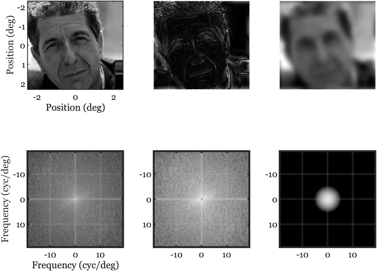
12.5 Two-dimensional Fourier Transforms representation
There are times when we would like to visualize the amplitude of the image harmonics as a function of spatial frequency. The image in Figure 12.8 is a common approach. The spatial domain images are on the left - two different harmonics. The amplitude of the Fourier coefficients are shown on the right. The center of the image represents the mean value. The two points, symmetric about the center, represent the amplitude of the Fourier representation.
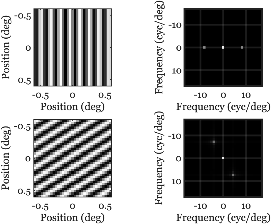
It is common to render the spatial frequency map with the mean (\(M\)) at the center \((0,0)\). In physical units, spatial frequencies span \([-f_N, f_N]\) along each axis, where \(f_N = 1/(2\Delta x)\) is the Nyquist frequency determined by the sample pitch \(\Delta x\). In index (DFT-bin) units for an \(N\times N\) image, frequencies run from \(-\lfloor N/2\rfloor\) to \(\lfloor (N-1)/2\rfloor\). Because the original image is real-valued, the Fourier coefficients obey \(F(f_x,f_y)=F^*(-f_x,-f_y)\).
Slow variations across the image are represented near the center of the spectrum. If we attenuate those low frequencies, the image emphasizes rapid variations (middle column). Conversely, attenuating high frequencies leaves a blurred version (right column).
12.6 System characteristics
The transform domain is frequently used in practice to summarize high level properties of image systems. Three important ideas, often expressed in the transform domain, are summarized here. These ideas have counterparts in the spatial domain as well, as they are system characteristics. They appear in the transform domain because they are easily expressed in terms of harmonics.
12.6.1 Image sharpness: High frequency roll off
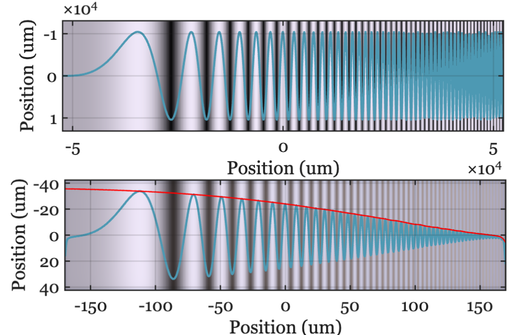
The apparent sharpness of an image is important in consumer photography applications. And the ability to resolve fine spatial details can be important in driving, robotics and other industrial applications. The system’s spatial resolution is usually determined by how well it encodes the high spatial frequency components of the image (Figure 12.9).
Natural images often exhibit amplitude spectra that decrease roughly as \(1/f^{\alpha}\) with \(\alpha\in[0.5,1]\). Optical systems further reduce high spatial frequencies due to diffraction and aberrations, reflected in the MTF roll‑off. As frequency approaches the system cutoff (e.g., the diffraction limit), contrast necessarily drops toward zero.
12.6.2 Spatial aliasing
When scene content contains energy above the sensor’s Nyquist frequency, it folds (aliases) into lower frequencies, producing artifacts such as moiré patterns. Anti‑alias strategies include optical prefiltering (defocus/diffusion), CFA design considerations, and oversampling followed by appropriate downsampling.
Maybe we illustrate it here in the abstract and then again when we get to the sensors, later.
12.6.3 Separability
One of the more interesting features of mathematical reasoning is the fact that there are properties present in higher dimensional analyses that have no counterpart in lower dimensions. A very simple, but important, example is the property of separability.
\[ F(x,y) = f(x) g(y) \tag{12.10}\]
How did we get to the close connection of imaging and the 2D Fourier Transform?
Sir William Bragg and Sir William Bragg (father and son) demonstrated that the pattern of X-rays scattered by a crystal is directly related to the crystal’s internal periodic structure. This led people to the understanding that the diffraction pattern is, in fact, the Fourier transform of the crystal’s electron density. This insight became a fundamental part of studying the 3D atomic structure of molecules. In fact, it led them to measuring the 3D diffraction pattern (the frequency domain data) and then performing an inverse 3D Fourier transform to get back to the spatial domain structure. A large part of crystallography became a practical problem of applied Fourier analysis.
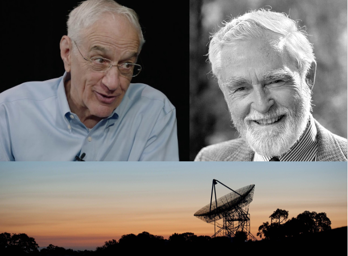
Ron Bracewell was an electrical engineer and applied mathematician who used his mastery of signal and imaging theory to revolutionize fields like radio astronomy and medical imaging. He developed the Projection-Slice theorem2, giving it a clear and elegant statement, and he wrote an important book, The Fourier Transform and Its Applications [1965],
Joe Goodman, was Bracewell’s colleague at Stanford. His main field is Electrical Engineering, with a profound specialization in optical information processing and statistical optics. Goodman’s important book, Introduction to Fourier Optics, educated a generation of physicists and engineers, cementing the 2D Fourier transform as the standard tool for analyzing optical systems, filters, and image formation.
In fact, the connection is even more direct: Joe Goodman was a student in Ron Bracewell’s course on the Fourier transform at Stanford. He has stated that Bracewell’s class “shaped my career,” and he dedicated one of his own books to Bracewell’s memory. Their work is a beautiful parallel: Ron Bracewell (an EE) applied Fourier analysis to understand and reconstruct images from radio waves (radio astronomy). Joe Goodman extended the mathematical methods to understand and manipulate light waves (optics).
Different fields use different terminology. Vision scientists often call these spatial frequency gratings. Engineers sometimes approximate sinusoidal patterns with evenly spaced bars or lines. We use the term harmonics.↩︎
The 1D Fourier transform of a projection of a 2D function is equal to a slice through the 2D Fourier transform of the function.↩︎