3 Measuring light
The book is still taking shape, and your feedback is an important part of the process. Suggestions of all kinds are welcome—whether it’s fixing small errors, raising bigger questions, or offering new perspectives. I’ll do my best to respond, but please keep in mind that the text will continue to change significantly over the next two years.
You can share comments through GitHub Issues.
Feel free to open a new issue or join an existing discussion. To make feedback easier to address, please point to the section you have in mind—by section number or a short snippet of text. Adding a label characterizing your issue would also be helpful.
Last updated: November 6, 2025
3.1 Measuring light: An overview
Imaging systems combine two tightly coupled parts: the acquisition hardware determines what is measured; the processing algorithms interpret the measurements. Effective image system designs optimize these components jointly. When we know precisely which aspects of the light field the hardware captures—over space, angle, wavelength, and time—we can build algorithms that make the best use of that information.
In this chapter we model light with rays for geometric reasoning, but a single ray is only an idealization with no energy. Real measurements always integrate over a finite bundle: a small area (or aperture), a small solid angle (direction range), a finite wavelength band, and a finite time interval. We may capture bundles diverging from a source or converging onto a surface; the same radiometric principles apply in either case.
Radiometry provides the quantitative framework for these measurements. We will work primarily with spectral (per-wavelength) quantities and SI1 units (e.g., watts or photons per second), which are standard in imaging and used by simulation tools such as ISETCam. The next sections define the core quantities — radiant flux, radiant intensity, radiance, and irradiance— and show how geometry (area, angle, and foreshortening) enters their units.
3.2 Radiometric units
Radiometric measurements are made separately for each wavelength. For people working in radiometry and image systems, wavelength is commonly expressed with respect to nanometers 2. We quantify the amount of radiance by measuring the amount of energy, or equivalently the number of photons, present at a location. The basic energy unit is joules per second, (watts) and for photons the basic unit is photons per second. Thus, in radiometry one often finds units such as (watts per nanometer) or (photons per sec per nanometer).
We describe the energy separately for each wavelength because, in most cases, the energy at different electromagnetic wavelengths act independently: we can measure the energy at two wavelengths separately, mix the two lights, and the result is simply the sum of the individual measurements. This additivity is a critical feature of light behavior in many cases 3 and is a foundational principle for many image systems (Section 29.2).
Radiometry defines units that are helpful for different types of geometry. The radiometric measures can be divided with respect to those from a source (radiance) and those arriving at a surface (irradiance). These can be further divided with respect to measurements from a small (point) source, or from an extended surface.
3.3 Photometric units
There is a set of units that summarize the impact of the radiation on the human visual system. These units are based on the spectral radiometry units, and we then calculate a weighted sum across wavelengths. The weights are selected to represent (roughly) the relative visibility of each wavelength. These photometric units parallel the radiometric units; for example, radiance and irradiance correspond to luminance and illuminance. In this section, we will describe the radiometric quantities. The experimental basis of photometry for the weighted sum across wavelengths -the key step to spectral radiometric quantities into photometric quantities- is explained in Chapter 24.
Part IV: Human Vision summarizes aspects of human vision that are important for image systems engineering. Please consult Foundations of Vision for more information about wavelength encoding and color appearance in human vision.
3.4 Radiance from a point
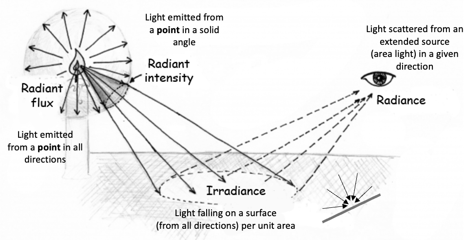
Figure 3.1 illustrates the geometry of four basic radiometric measures. The upper left illustrates a point source. The radiant flux measures the total energy emitted from the point in all directions. As for all radiometric measurements, the energy (watts) is specified as a function of wavelength (watts/nm).
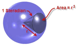
Often, we measure the light emitted by a point source in a particular direction, the radiant intensity. In that case we measure the energy within a cone of rays in a particular direction. The standard unit for angles in three-dimensions is the steradian, just as the radian is the standard unit for angles in two-dimensions. The radiant intensity has units of watts per steradian per nanometer (watts/sr/nm). Thus, if the measurement instrument measures energy over an angle of 0.5 steradians, we divide the measurement by 0.5. If the instrument sums over 10 nm bands, we divide the energy by 10. In this way, the radiant intensity normalizes the angle we measure to the unit steradian and per nanometer. The standard symbol for radiant intensity is \(I(\lambda)\).
3.5 Radiance from a surface
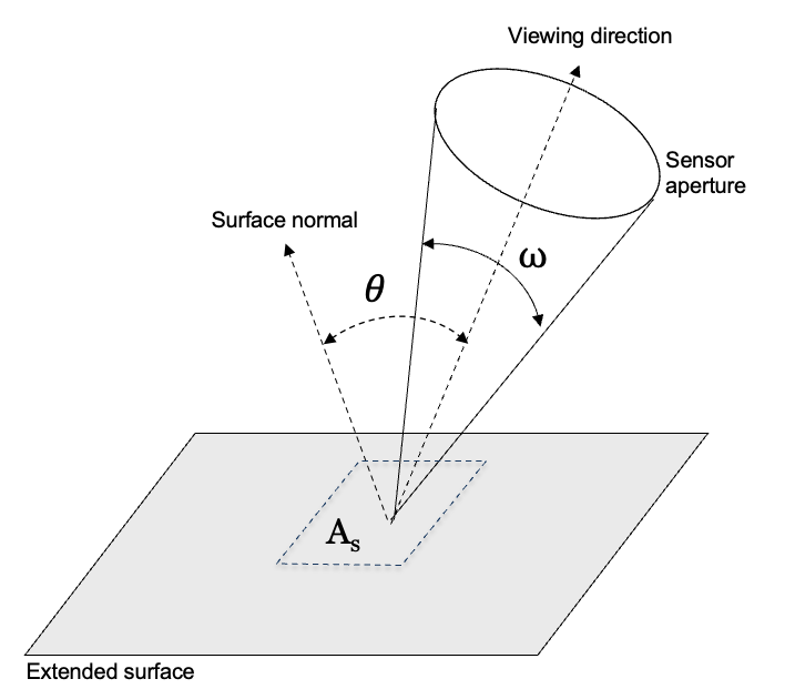
In many applications we measure radiance from a patch on an extended, flat surface - such as a large light fixture with a diffuser, a wall, or a large display screen. The geometry of such a measurement accounts for two main factors illustrated in Figure 3.3. First, we must account for the area of the surface patch, as seen from the detector. For example, if the measured surface patch is a square \(0.1\) meters on a side its area is \(A_s = (0.1~m)^2\). The area of this patch, as seen from the detector, is foreshortened. We calculate the foreshortened area using the angle between the viewing direction and the surface normal, \(\theta\), which becomes \(A_s \cos(\theta) ~ m^2\). Second, we account for the size of the bundle of rays captured by the detector. We measure this size by its three-dimensional angle, \(\omega ~ sr\), from a surface point that will be measured by the detector. The radiance combines the energy measured at the sensor (\(watts/nm\)) with these geometric factors. The standard symbol for spectral radiance is \(L(\lambda)\). It has units of watts per nanometer per unit foreshortened-area per steradian:
\[ \frac{Watts}{nm ~ \cos(\theta) ~ m^2 ~ sr} \]
3.6 Radiance from a large surface
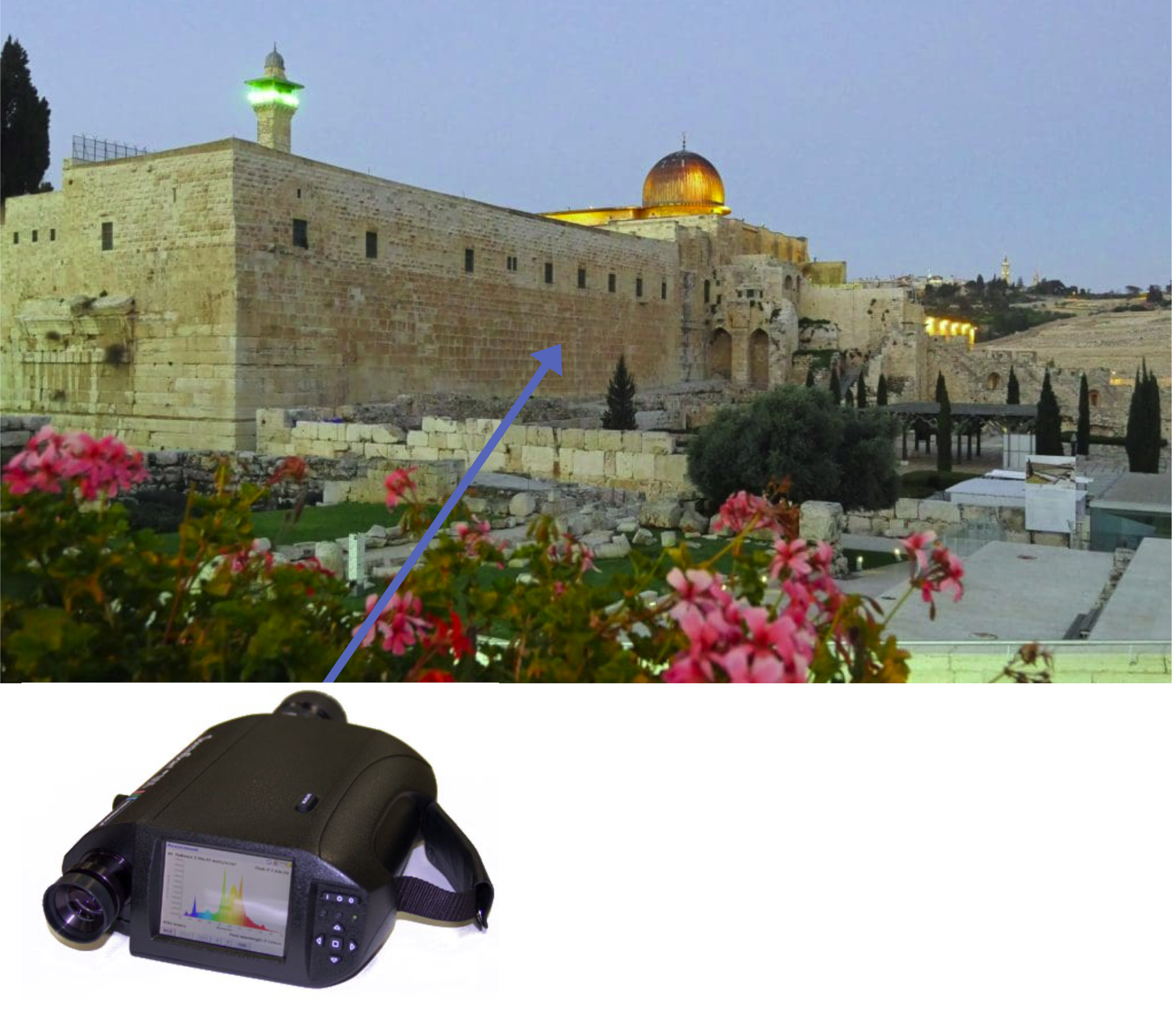
Measuring the radiance from a large wall with a spectroradiometer. The distance from the wall does not impact the measurement. Why?
Explain the different panels a bit here, and the tradeoff.
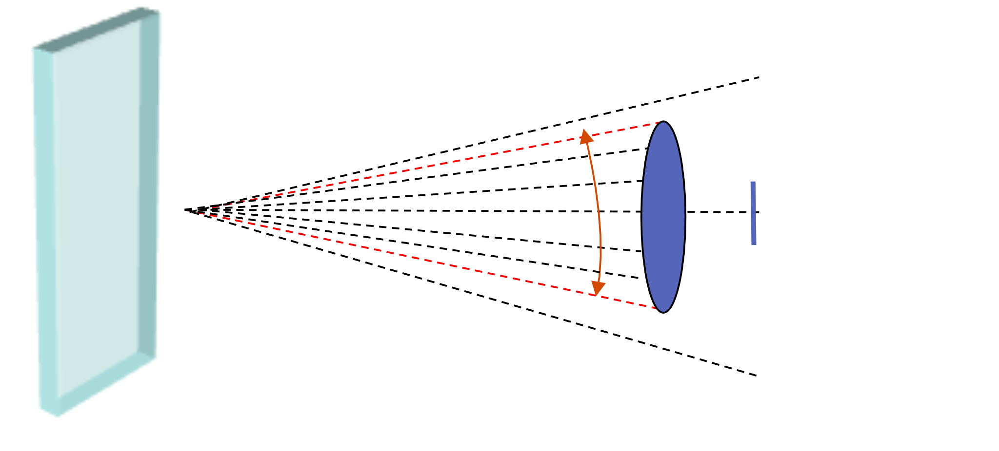
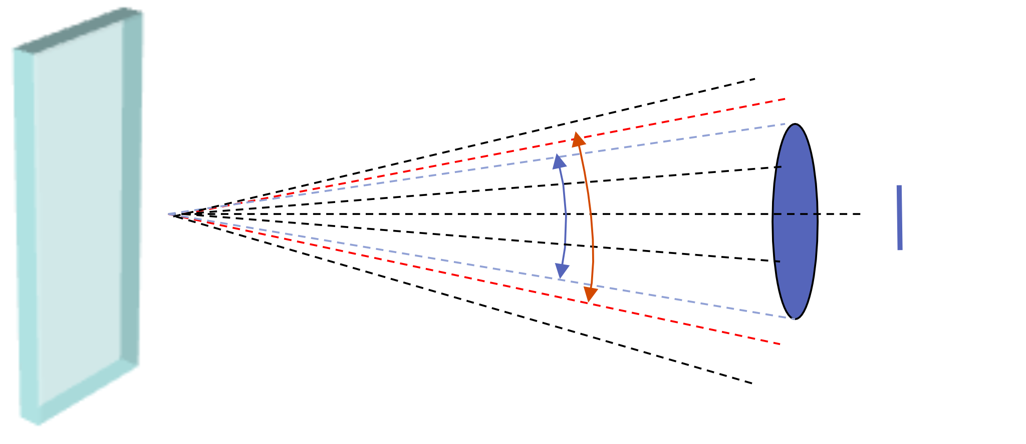
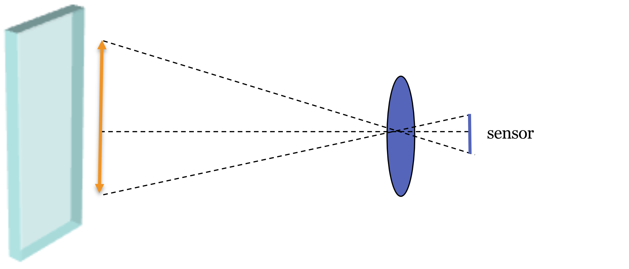
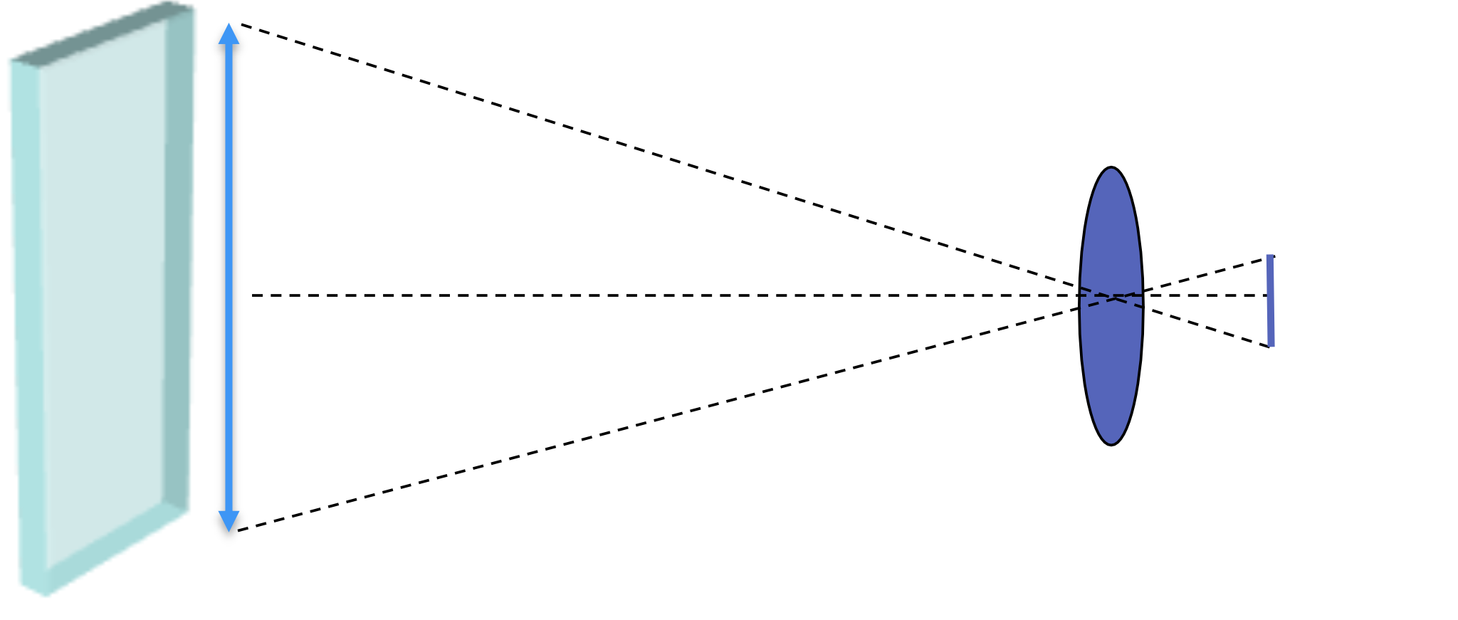
Here is a tabular summary of the tradeoffs - solid angle and contributing surface area cancel one another. If the wall is uniform, then the distance will not matter.
| Parameter | Distance |
|---|---|
| Solid angle | Decreases |
| Surface area | Increases |
3.7 Irradiance on a surface
Another important measurement is the radiance incident upon a surface, the irradiance. This quantity is important to calculate the radiance available to an image sensor or the retina. It is also a practical measure in assessing room lighting, say how much light will arrive at a desk top. The irradiance sums the energy arriving from all directions, hence no three-dimensional angles (steradians) are specified. The irradiance measures the total energy per unit area of the surface. The standard symbol for irradiance is \(E(\lambda)\), has units \(watts/nm/m^2\).
The amount of light from a small source, say a point source or a light bulb, that irradiates a surface depends on the geometry relating the light source and the surface. Figure 3.6 illustrates two cases: the same angular rays emerging from both light bulbs. On the left the surface is perpendicular to the direction of the central ray. On the right, the surface is slanted and not perpendiulcar; th same bundle of rays is spread across a larger surface area. Thus, there will be less light per unit area when the surface is not perpendicular to the main ray. In the most extreme case, when the surface is parallel to the central ray, no light will fall on the surface at all.
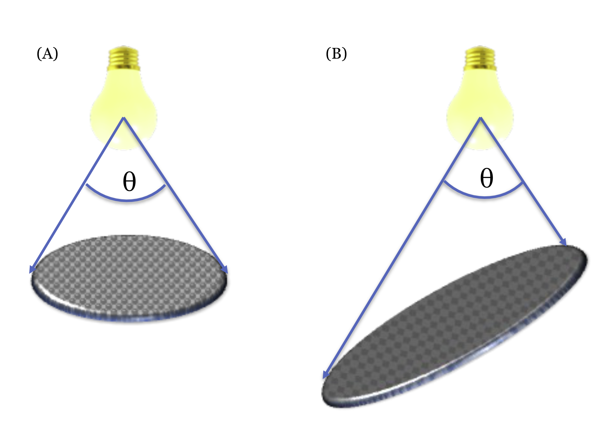
The geometric relationship between surfaces and relatively small light sources in an image is an important part of rendering images in computer graphics and measuring the illumination on surfaces in natural settings. The geometric factor illustrated here is complementary to the geometric factor illustrated in Figure 3.3 for how we measure the light radiating from a surface.
3.8 Radiometric units
Figure 3.7 is a guide to help you remember the four fundamental spectral radiometric measurements. Please note that people will sometimes report a measure of any of these radiometric quantities by summing the energy across all wavelengths. This would be called, for example, the total radiance or total irradiance, rather than the spectral radiance. I list the corresponding photometric measurements in Chapter 23. The photometric values are also a sum across wavelengths, but weighted by the relative visual significance of the different wavelengths.
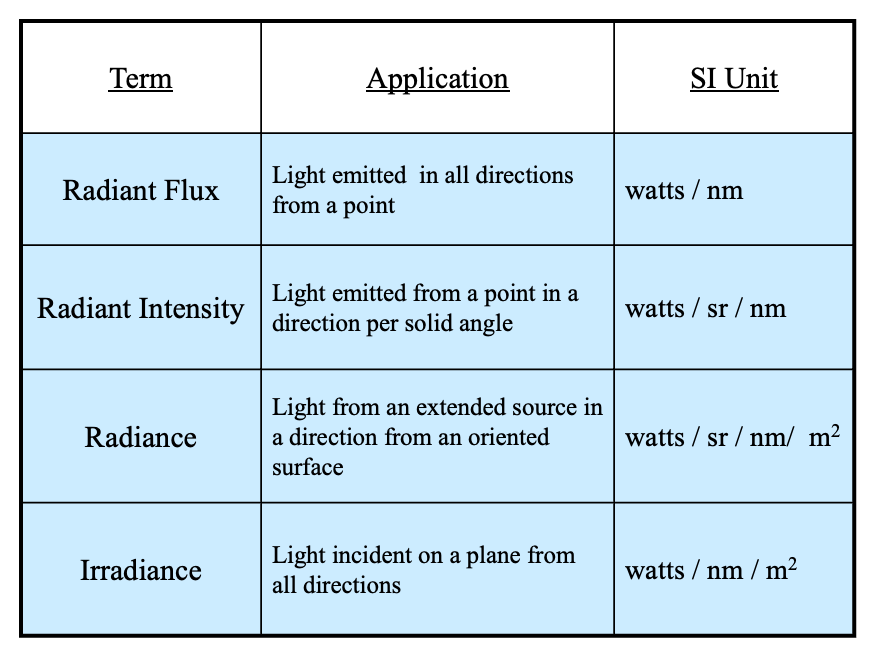
How do we determine whether we are measuring a part of a surface or a point? The distinction between measuring a surface and a point source is not always clear-cut. Here are some principles, though none is definitive.
- Distance: If the distance to the source is significantly larger than the dimensions of the source itself, it can be approximated as a point source.
- Solid Angle: If the solid angle subtended by the source at the detector is very small, it can be approximated as a point source.
- Precision: If high accuracy is required, it’s generally better to use the radiance formula, even for small surfaces. This allows you to account for the angular distribution of the emitted radiation. If lower accuracy is sufficient, and the source can be reasonably approximated as a point source, the radiant intensity formula can be used.
These recommendations are filled with imprecision that I always try to remove. They contain words, like ‘small’, ‘large’, ‘high’, and ‘low’ because there is no fixed threshold at which a surface definitively becomes a point source. It is your decision whether to treat the source as a point. What is important is to tell people exactly what you did. If they don’t like your choice, they can do it their own way. Or they can ask you - nicely - to try it another way.
3.9 Beyond the basics: BRDF, light field, colorimetry
The four fundamental radiometric measurements provide a foundation for understanding light. In later chapters, we will expand on these concepts by introducing additional factors.
A key extension is directional dependence. Radiance from a surface patch varies with viewing direction and is often written as \(L(\mathbf{x}, \omega, \lambda)\), where \(\omega\) denotes direction using polar angle \(\theta\) (from the surface normal) and azimuth \(\phi\). Likewise, the irradiance at a surface point is the directional radiance integrated over the hemisphere, weighted by the cosine-foreshortening factor, \[ E(\mathbf{x}, \lambda) = \int_{\Omega^+} L(\mathbf{x}, \omega, \lambda)\,\cos\theta\, d\omega. \] These angle-dependent behaviors are central to how materials reflect and transmit light. We will study them with the bidirectional reflectance distribution function (BRDF), \(f_r(\omega_i,\omega_o,\lambda)\), in Section 5.8.
The properties of modern image sensors also add practical constraints. Sensors are 2D arrays of small light-sensitive elements (pixels) that spatially sample the irradiance at the sensor plane. Each pixel integrates photons over its finite area, over the exposure time, over wavelengths weighted by its spectral sensitivity, and over the acceptance cone set by the lens and pixel aperture. Pixel counts, and the corresponding microlens arrays, have grown from early arrays with a few hundred by a few hundred pixels to today’s sensors with tens of millions.
Capturing directional information—measuring rays from different directions separately, as in Figure 2.7—yields richer data and is the basis of light field imaging. The geometry of pixels, including small lenslet arrays placed over the pixel arrays, enables us to make useful measurements about the light field.
Similarly, reproducing color requires pixels with different wavelength sensitivities (e.g., a color filter array). The idea that we can use just three measurements to represent human color perception was formalized in Maxwell (1872) and led to the field of colorimetry, which we will explore in Part IV: Human vision.
Système International d’Unités. These units are the modern form of the metric system, the most widely used system of measurement in the world.↩︎
Units of micrometers (microns, \(\mu\)) are commonly used by people working in the infrared studies, units of angstroms in atomic and x-ray studies, and electron volts in high-energy photon research.↩︎
There are important cases light when radiance at one wavelength evokes emissions at a different wavelength (fluorescence). There are also important cases of non-linear behavior (e.g., two-photon imaging). We discuss these when we review special instrumentation. But the vast majority of image systems are linear and the Principle of Superposition applies (Equation 29.1).↩︎