22 Human spatial encoding – Foundations of Image Systems Engineering

22.1 Human spatial encoding overview

The image systems components we studied in earlier chapters have a structure that has an input and an output. This makes it possible to characterize these systems using transfer functions, such as the OTF and pointspread. The human visual system does not have an output that we can measure directly; the percepts we experience are private. Consequently vision science has relied on a wide variety of measurements, some direct and some indirect, to make inferences about the neural processing that underlies human perception.

In the first part of this chapter, I review how blurring by the optics and sampling by the photoreceptors limits the spatial resolution. These measurements characterize only the first steps in seeing, but they are important because they represent a bottleneck. Spatial information that is not captured by the eye can only be guessed at by the brain.

There is more information available in the cone photoreceptor array than we effectively process. The neural processing strategies that interpret the image do not aim to use every scrap of available information. This gap is of interest, of course, for image systems engineers who are interested in predicting human perception, such as perceived image quality. Information about the spatial resolution of human performance must come from measures of this performance. Some of these measurements are amenable to quantification and they can be used to create quantitative engineering metrics (e.g., Barten’s model).

There are many other measurements that are useful for revealing the principles implemented in the neural processing, but not immediately applicable to image systems evaluation or design. The material in this section describes measurements that are relevant to engineering metrics, and the material in Foundations of Vision includes many more measurements that are helpful for understanding the general processing strategies.

22.2 The Two Stages of Encoding

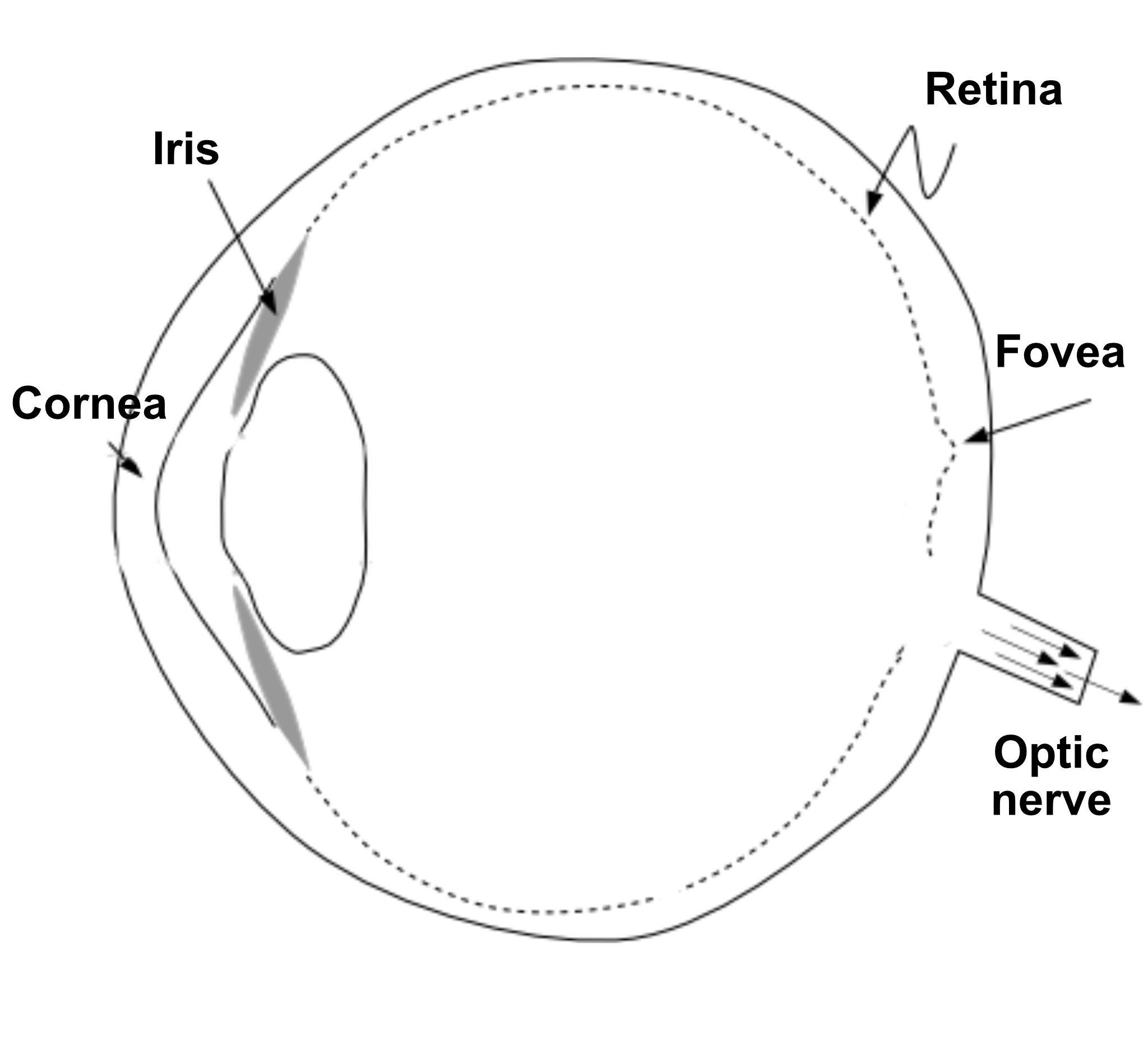
Two systems in the eye function together to convert electromagnetic radiation from the scene into a neural signal that the brain interprets (Figure 22.1).

First, the physiological optics—the cornea and lens—act like a camera lens. The optics gathers the radiation entering the eye and focuses it to form an image on the retina. This optical system transforms the radiation from the environment into a focused optical image.

Second, the retina, a thin layer of neural tissue lining the back of the eye, contains a set of highly specialized neurons that convert this optical image into neural signals. This process, called transduction, is performed by the photoreceptors. The signals from the photoreceptors, in the form of synaptic transmitter release, are processed by several distinct networks of retinal neurons. The output of these networks is sent to the brain on the axons of the retinal ganglion cells (RGCs). The bundle of RGC axons exit the retina through a small hole and form the optic nerve.

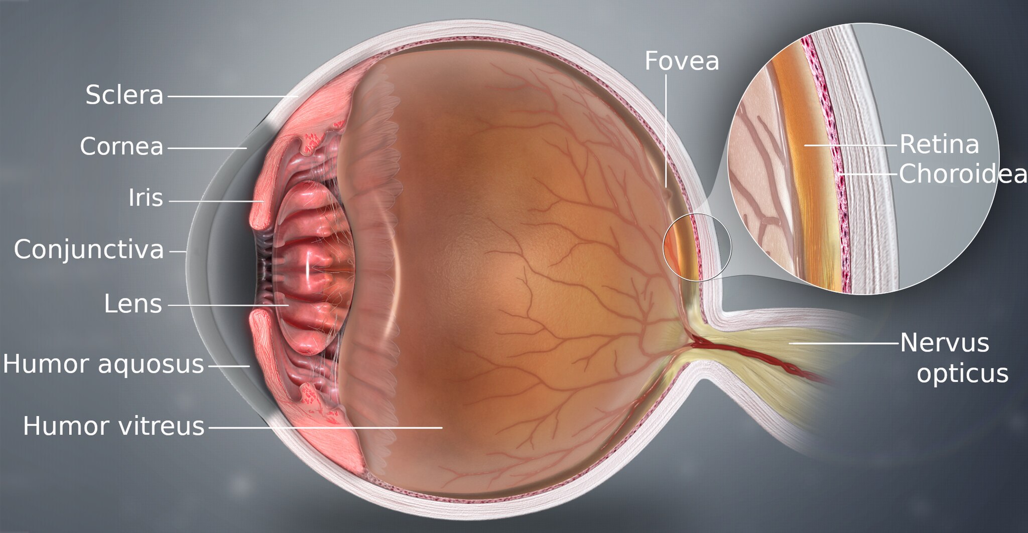
(a) A cross-section of the human eye, showing the cornea, lens, iris, and retina.

The retina is a feed-forward system; there is no direct neural feedback from the brain. This simplifies our work, allowing us to study the retina’s input-output relationship without accounting for top-down signals—a luxury we rarely have when studying other parts of the brain.

However, the brain does send signals to the eye that control pupil size and lens power. It also controls eye, head, and body positions, determining which part of the visual world falls on the retina. These signals do not reach the retinal neurons directly, but they are essential for seeing.

22.3 Physiological optics

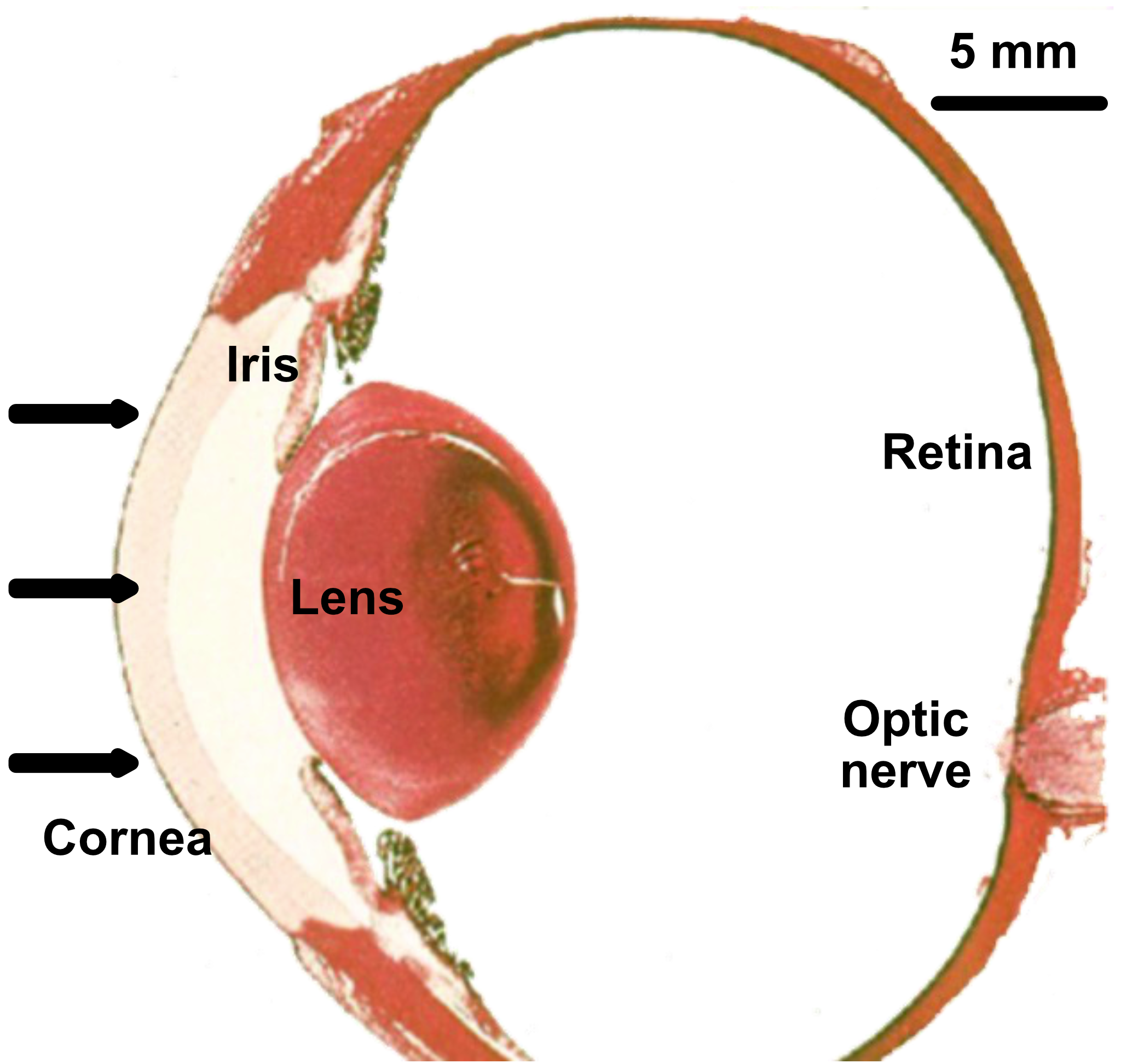
The cornea and the flexible lens work together to focus light, forming an image on the retina, as shown in Figure 22.3. This optical system is dynamic, constantly adjusting both the amount of light it lets in and its focal length.

The amount of light entering the eye is controlled by the pupil, an aperture that can dilate (open) to about 8 mm in diameter in dim light or constrict (close) to about 2 mm in bright light. This change in area adjusts the light intake by a factor of about 16 (or 1.2 log units). While significant, this is a small adjustment compared to the vast range of light levels we encounter in nature, which can span as much as 10 log units across a single day. The pupil’s size changes automatically in response to light, but it is also influenced by cognitive and emotional states, such as arousal or mental effort.

The pupil size also determines which part of the cornea and lens contributes to image formation. When the pupil is constricted, the image is formed using only a relatively small central part of the cornea and lens. Under these conditions, optical aberrations are minimized, and the image quality can be very high, sometimes approaching the diffraction limit. When the pupil is wide open, a much larger region of the cornea and lens is used. Because biological optics are not perfect, aberrations become more significant, and the image quality is far from diffraction-limited.

The eye changes the object plane that is in focus through a process called accommodation. Neural signals control the ciliary muscles, which are connected to the lens by the zonule fibers. To focus on nearby objects, the ciliary muscles contract. This contraction reduces the diameter of the ring they form, relaxing the tension on the zonule fibers. This allows the elastic lens to become more rounded (convex), increasing its optical power. To focus on distant objects, the ciliary muscles relax. This increases the diameter of the ring, which pulls on the zonule fibers and flattens the lens, decreasing its optical power.

This lens flexibility is not permanent. With age, the lens gradually stiffens, reducing its ability to change shape. This condition, known as presbyopia, makes it difficult for older people to focus on near objects. The loss of near-field visual acuity typically becomes noticeable in one’s early to mid-40s and is a natural part of aging, commonly corrected with reading glasses. It happens to all of us.

22.4 Retina

Since the 1990s, vision scientists have been able to measure the quality of the physiological optics. Below, I describe the techniques invented to make these measurements. The Appendix explains how we use these measurements and ISETBio to simulate the transformation of the incident light field into the retinal image.

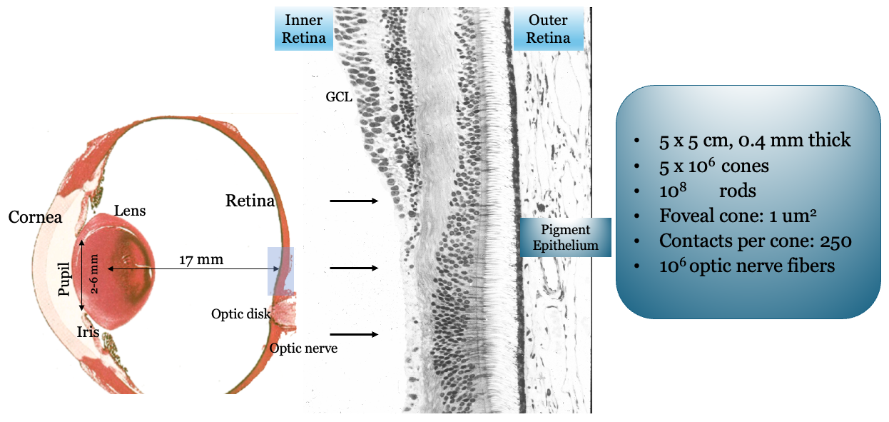
It is important to understand these optics in terms of the photoreceptor sampling array. A 5-micron optical spread has different implications if sampled every 2 microns versus every 10 microns. Thus, before discussing physiological optics, we consider the retina and the photoreceptor mosaic.

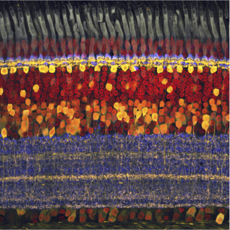
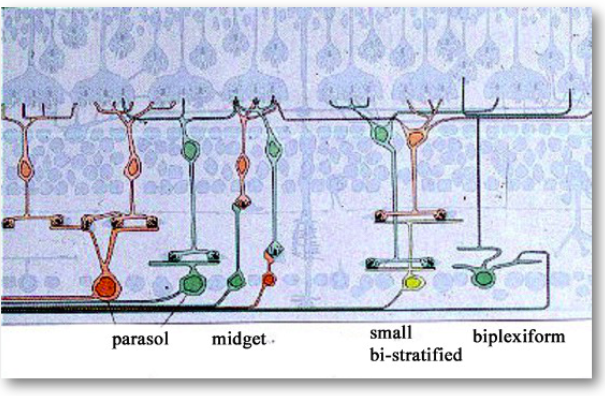
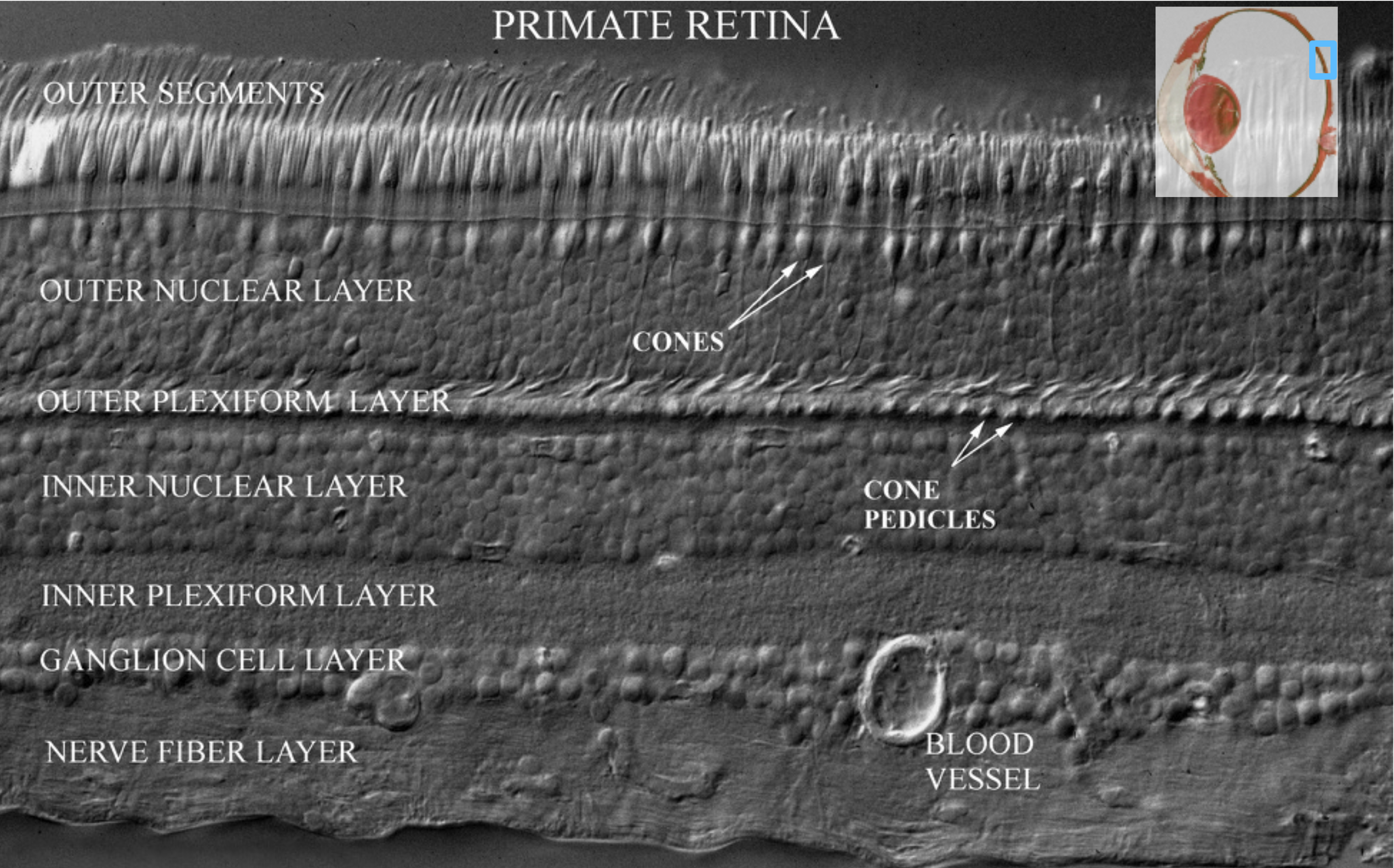
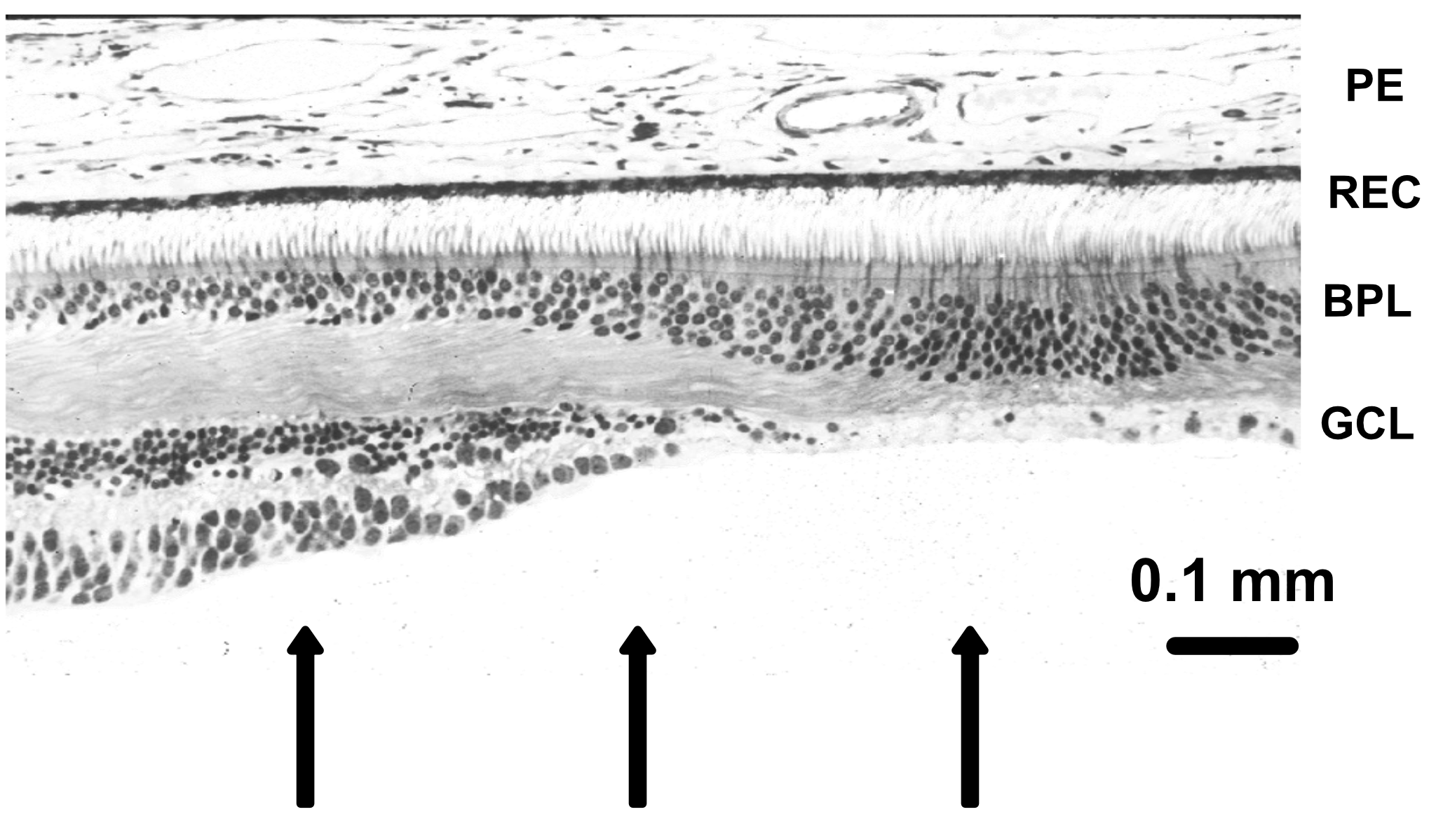
The retina is approximately \(200–300\) microns thick near the posterior pole, varying from about \(100\) to \(500\) microns across the retina. Its total area is on the order of \(10–12~cm^2\). It is a laminated neural tissue comprising three nuclear layers separated by two plexiform layers. There are on the order of 80 different cell types that can be identified through their genetic expression, responses to light, and anatomical form. The retinal cells form stereotyped connections, which we call retinal circuits. We believe that there are about 20 such circuits. The circuit outputs, carried on the retinal ganglion cell axons in the optic nerve, project to a variety of locations in the brain.

The vast majority of light-driven activity is initiated in the photoreceptors (rods and cones). The rods are the dominant source under very low light levels, and the cones are the dominant source under moderate to high light levels. The typical retinal circuit is driven by activity that starts in a local region of the photoreceptors. The same basic circuit will be present throughout the retina, tiling the photoreceptor mosaic, though the absolute size of the cells and their input regions generally vary across the retina. The size of the region increases as one measures from the highly specialized central fovea into the periphery.

There is one important and interesting exception, only recently discovered. There exists a class of retinal ganglion cells that contain a light-sensitive pigment (melanopsin). These cells, called the intrinsically photosensitive RGCs (ipRGCs), absorb photons and respond to overall light level. There are not a lot of these cells, but their outputs are important for circadian rhythms and pupillary control. They may also influence other aspects of vision.

(a) This image shows the different layers of the retina very clearly. The different cell types are stained with different materials. Source: New Scientist

22.5 Adaptive optics

In the late 1990s, it became possible to measure how the physiological optics blurs the light in the living human eye. A key technology for making this measurement is adaptive optics, based on a measurement device called the Shack-Hartmann (S-H) wavefront sensor. This wavefront sensor was originally developed by astronomers pointing their telescopes at the stars. They knew that the wavefront from space was distorted by the atmosphere. They developed the sensor and adaptive optics system to measure the wavefront distortion and correct it.

The principle of the measurement is illustrated in Figure 22.4. A narrow beam of light is directed through the center of the pupil. Some of the light is reflected from the retina, at the layer between the inner and outer segements of the receptors. The reflected light is Lambertian (spread in all directions) and fills up the lens as it passes back through the optics. If the optics were perfect, the rays exiting the eye from the small spot would be close to collimated and the wavefront would be a constant. But the rays are not parallel and thus the wavefront has some deviations from constant. These are the aberrations that we measure at the S-H wavefront sensor. They are introduced by the optics of the eye.

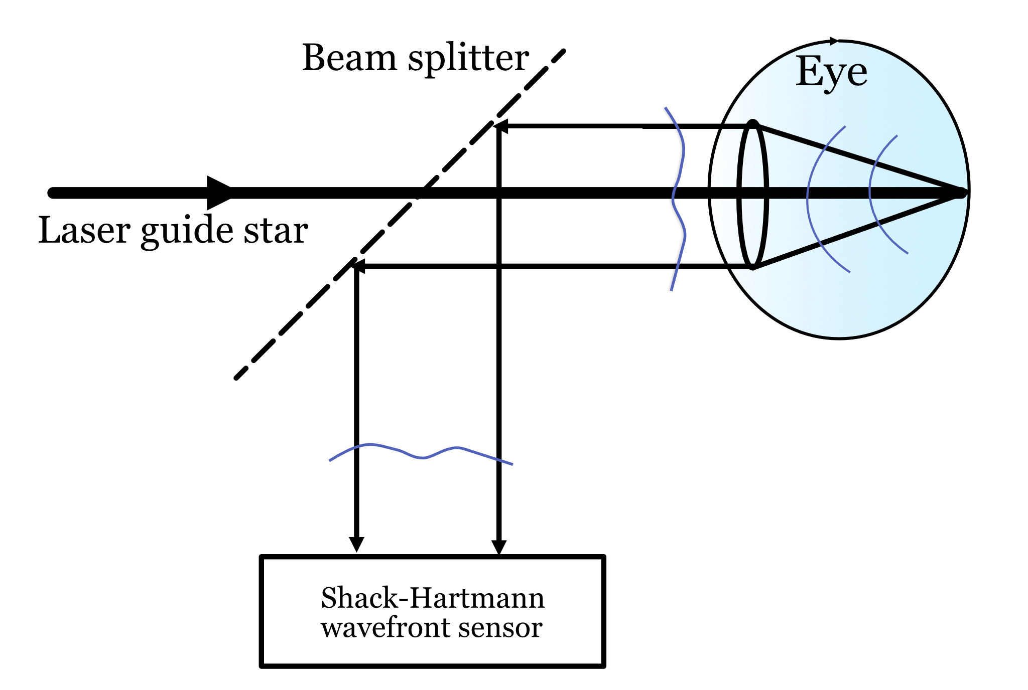
In addition to measuring the optics, the S-H wavefront sensor enables to additional functions. First, we can use knowledge of the wavefront distortion, to create a very sharp image at the back of the eye. We do this by pre-distorting the rays of our image before they pass through the optics. This way, the effect of the optical aberrations is to cause the reflected rays to be without any distortion and thus the image is diffraction limited. Such an image can be localized to a small spot, exciting just a single cone.

Second, we can use the method to create a relatively sharp image of the retina. When the pupil aperture is fairly large, say 7 mm diameter, the diffraction-limited PSF (Airy disk) will have a small diameter of about 3 microns. Scanning a spot across the retina provides an point-by-point image of the back of the eye, blurred only by the 3 microns of the Airy disk. This technique, called adaptive optics - scanning laser ophthalmoscope (AOSLO)- enables us to form a crisp image of many parts of the photoreceptor mosaic.

Shack-Hartmann

22.5.1 Shack–Hartmann wavefront sensor

Johannes Franz Hartmann was a German astronomer working on the problem of detecting optical defects in telescope objectives. Reasoning from the ray theory of light, he measured the optical light field from a simple stimulus: an on-axis point at the focal length of the lens. In principle, the rays emerging from an ideal lens would all be parallel to the main axis. To measure deviations from the ideal, he created a screen comprising an array of pinholes. If the rays exiting the lens were parallel, the light through each pinhole would create a spot that is nicely centered behind the pinhole. If the rays from the lens were not parallel, the image behind the pinhole would be displaced by from the center. The measured displacements could guide how the lens might be improved.

In practice, the image from each pinhole produces a blurry spot due to diffraction. Thus Hartmann did not try to extract an image; he just estimated the central position of the blurry spot. Also, because the pinholes only let through a small amount of light, the technique was not very sensitive.

Hopefully these ideas are familiar to you by now - it is the same principle we used when describing the light field measurements (Section 2.7, Figure 2.7). Because there is an array of these pinholes, the accumulation of pinhole images measures the rays at multiple angles at multiple positions. In principle, by performing this measurement for different wavelengths and polarizations, we sample the optical light field (Equation 2.3).

Arizona History of the Shack work.

22.6 Photoreceptor types

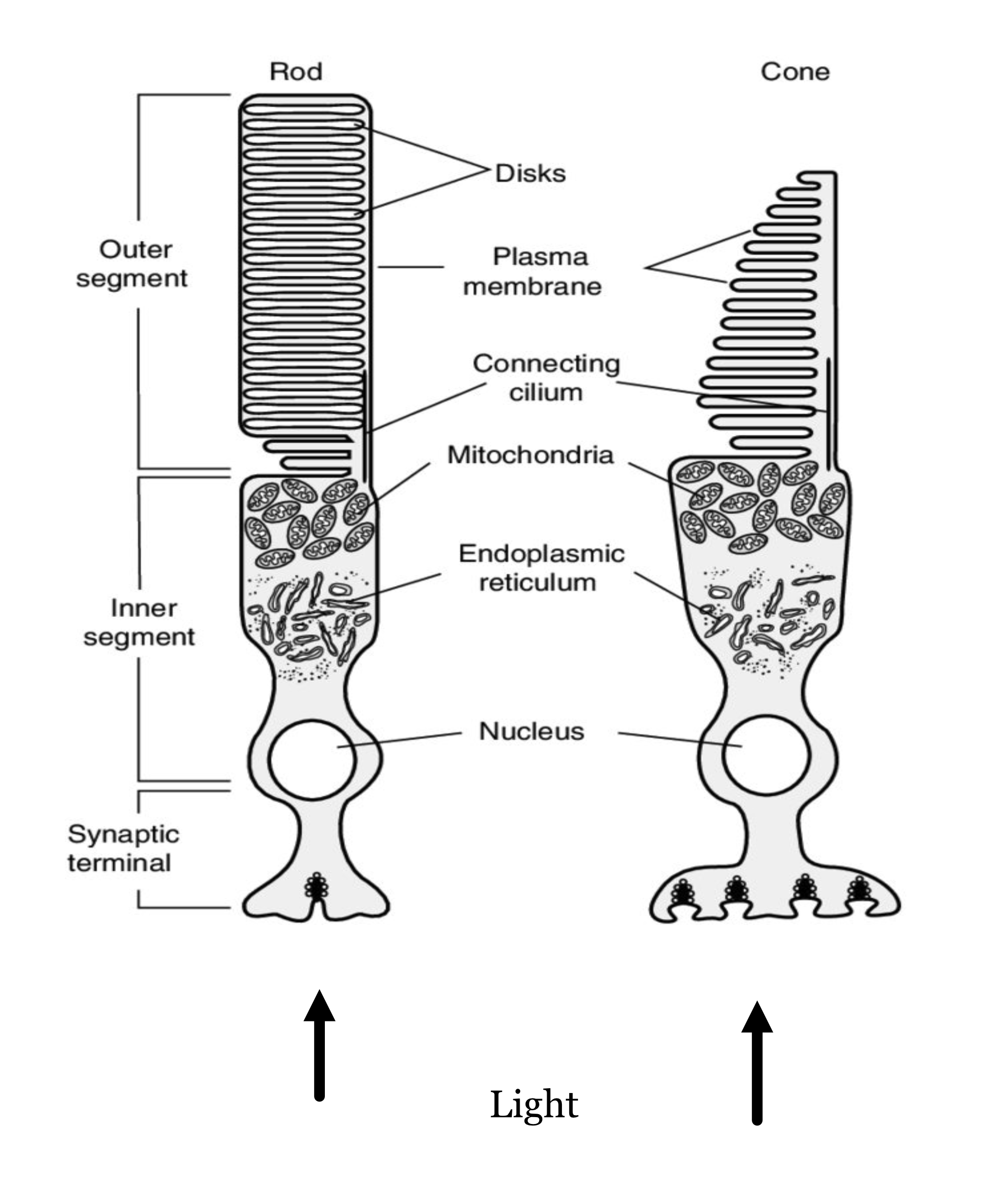
The rod and cone photoreceptors are specialized neurons whose principal function is to convert electromagnetic radiation into a neural signal. Both types of photoreceptors accomplish this using a light-sensitive pigment (photopigment). This pigment absorbs photons and, in so doing, initiates a chain reaction of events within the cell (Stryer (1986)). These events, the transduction cascade, result in a change in the synaptic signal from the photoreceptor. The spatio-temporal pattern of changes across the photoreceptor mosaic is the signal that the nervous system interprets and the basis of our sight.

The arrows at the bottom indicate the direction of the incoming light (the lens is below). The light arrives at the photoreceptor layer, brought into focus by the physiological optics. Some of the light enters the cell through the inner-segment aperture. Because of the refractive-index contrast between the inner segment and surrounding medium, the inner segment acts as a waveguide that directs the light toward the outer segment, where it initiates the transduction cascade.

(a) Denis Baylor’s Proctor Medal award included this very simple diagram, which he entitled ‘A physiologist’s diagram of a rod and cone.’ The horizontal lines show the stacks of photosensitive pigment molecules within the outer segment of these cells. The arrangement differs between the rods and cones. In the rods, the photopigment is mainly contained in discs (saccules) that are not continuous with the cell’s surface membrane. In the cones, the photosensitive membrane is continuous with the cell surface. 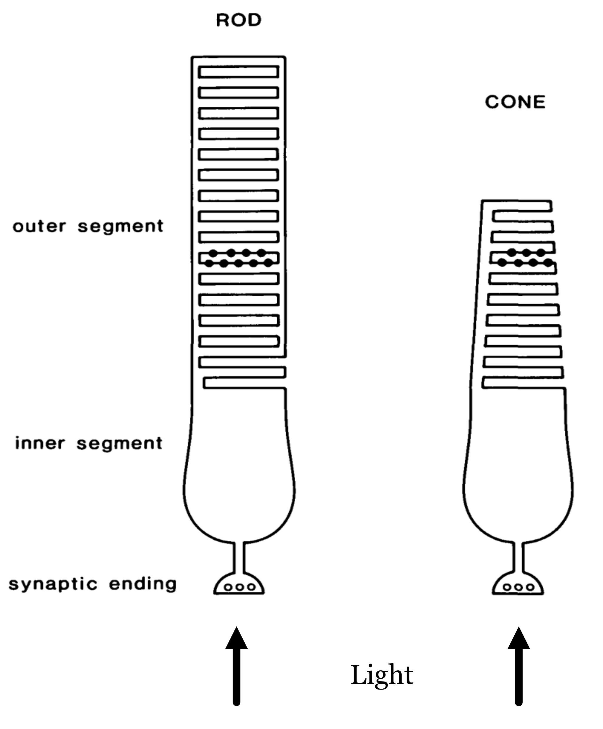The absorption of a photon initiates a series of events (transduction cascade) that modulates the membrane potential and the rate of synaptic transmitter release. The transmitter itself is packaged in synaptic vesicles, shown by the circles. Source: Baylor (1987)

The rod and cone photoreceptors are two largely distinct systems. The rods are mainly used to provide vision under low light levels (scotopic; e.g., nighttime). There is only one type of rod photopigment, rhodopsin. For this reason the rod system provides no information to compare the different wavelengths of light incident at the retina.

The cone photoreceptors dominate vision at modest to high levels of illumination. There are three types of cones, containing three different photopigments. These photopigments absorb over a fairly broad wavelength band, but they have different peak sensitivities in the long-, middle-, and short-wavelength parts of the visible spectrum. I will cover more on this in the color section below.

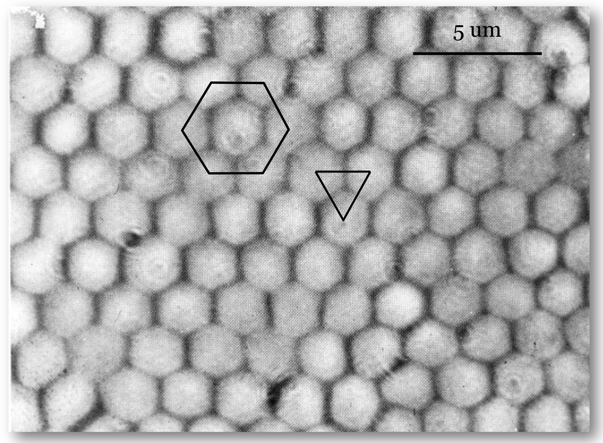
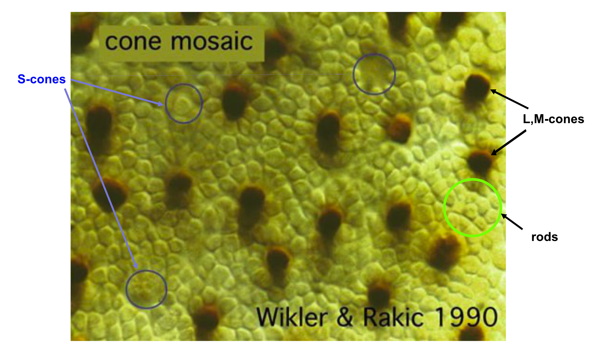
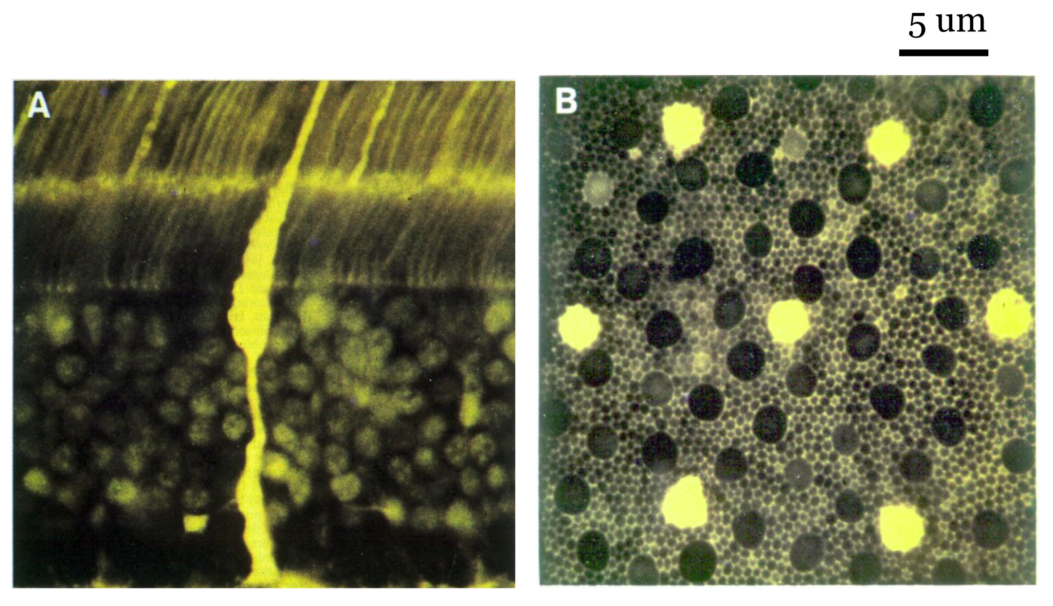
The spatial resolution of the human eye depends on the aperture size and spacing of the photoreceptor inner segments, particularly for the cones. A great deal was discovered about the sampling mosaic in the 1980s and 1990s Curcio et al. (1990). Prior to that time, the nature of the cone sampling mosaic and the importance of sampling were not widely appreciated. The importance of sampling was emphasized by Yellott and colleagues, who analyzed the spatial sampling. William Miller and Joy Hirsch, at Yale, were among the first to crisply show the dense packing (Hirsch and Miller (1987)). Over small patches of the primate retina the packing is quite dense (Figure 22.6), in a spatial arrangement called a triangular (hexagonal) packing.

Figure 22.6: Cone inner segment spatial sampling. Source: Hirsch and Miller (1987) (personal communication)

How does the spatial sampling of the cones compare to the optical PSF? One comparison we can make is for the central fovea. There the inner-segment apertures are about 1.5–2 microns in diameter. Using ISETCam we can calculate the diffraction-limited Airy disk diameter (first minimum) for a 550 nm light. For a 3 mm pupil, the f-number of the human optics is 17 mm / 3 mm ≈ 5.6. Using Equation 7.2, this is:

>> radius = airyDisk(550,5.6,'units','um','diameter',true)
radius =
    7.5152

This calculation shows that a tiny point in the scene -say star light- will be spread over a diameter of about 7 \(\mu\text{m}\) on the retinal surface, which corresponds to a 3 or 4 foveal cones. In natural vision, therefore, no stimulus will excite a single photoreceptor; the nervous system always receives signals from multiple cones, even if it draws the inference that the source is a single, very tiny point of light.

One reason for creating such a system that spreads the light over several cones may be to enable us to judge the wavelength information. It is likely that spreading the light across 5-10 cones will engage cones with more than one type of photopigment, and the relative excitation of the different types of cones is the signal we use to judge color. We encountered a similar principle when describing the color filter array in cameras; designers purposefully introduced some blur so that any small region of the scene would engage the R,G and B pixels (Section 17.3.2).

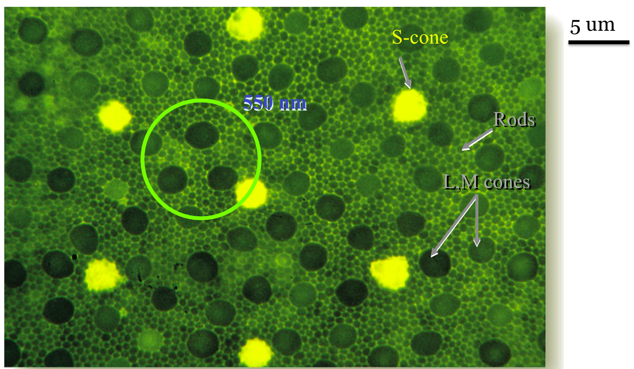
What is the arrangement of the different cone types in the human eye? Some data on this point emerged in the 1980s and 1990s when biologists discovered fluorescent markers that would attach to just one type of photoreceptor (DeMonasterio et al. (1981), Monasterio et al. (1985) Wikler and Rakic (1990)). These measurements could distinguish the L,M cones from the S-cones.

(a) L,M cone types, intermixed with rods, and some S-cone hints. Lots of rods. Near periphery. Source: Wikler and Rakic (1990)

About ten years later, new estimates that could distinguish between the L- from M-cones were obtained in the living human eye. These measurements used adaptive optics coupled with knowledge about the relative wavelength selectivity of the different cone types (Roorda and Williams (1999), Hofer et al. (2005), Hofer and Williams (2014)). I explain these measurements in the Foundations of Vision, 2nd edition. When that gets written.

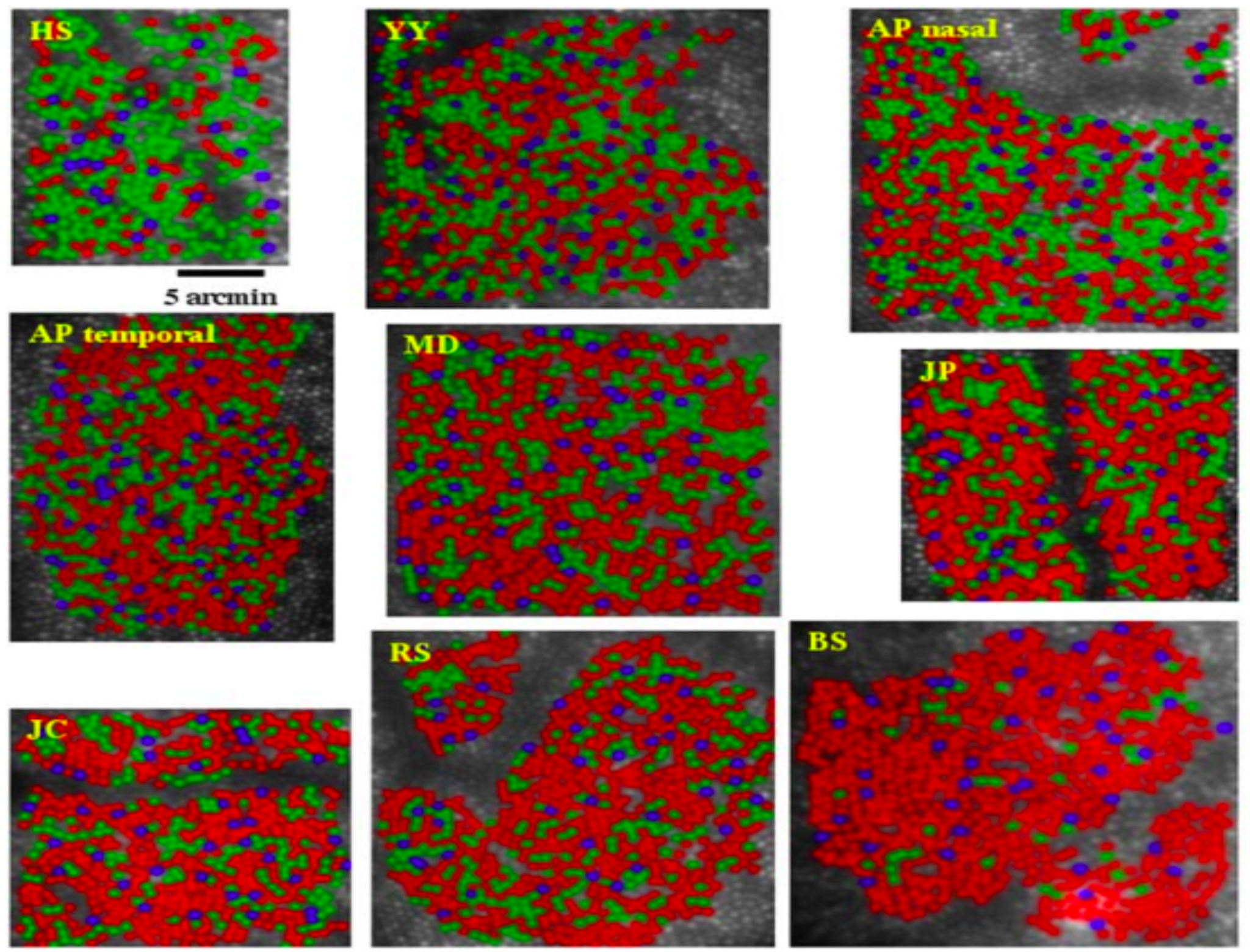
Figure 22.8: Source:Hofer et al. (2005), Figure 4

These measurements revealed something that was quite surprising to vision scientists: the ratio of L- to M- cones in the living human eye differs greatly between people. Some of us have equal numbers of L- and M- cones, while others have a large predominance of L-cones. To this point in time, we have not learned how to measure these differences in behavioral experiments, although there have been some attempts. I suspect that an enterprising engineer or scientist will find a means to do so in the future. One of the reasons that the difference is hard to reveal is that the L- and M-cones are so similar to one another.

22.7 Cone mosaic at different eccentricities

The cone spatial sampling density and inner segment aperture size varies a great deal between the fovea and periphery. In the central fovea, the cones are tightly packed and their inner segment aperture diameters are very small (1-2 microns). In the periphery the cones are much more widely spaced and their inner segment apertures are nearly ten times larger (Figure 22.9). Hence, our encoding of the retinal irradiance is very different between the fovea and periphery.

TODO: Incorporate Watson estimates for RGC density, as well.

TODO: There is an ISETBio figure related to s_coneEccentricities.m that we could reference and include as a fise_<> file.

(a) Simulation centered on the fovea. Notice that there are no S-cones in the very center and no rods throughout.

22.8 PSF at the cone inner segments

We are now ready to describe the optical spread with respect to the cone spatial sampling. First, we illustrate for a typical person how the PSF changes with visual field eccentricity. Second, wwe illustrate how the PSF changes with wavelength.

22.8.1 Eccentricity dependence

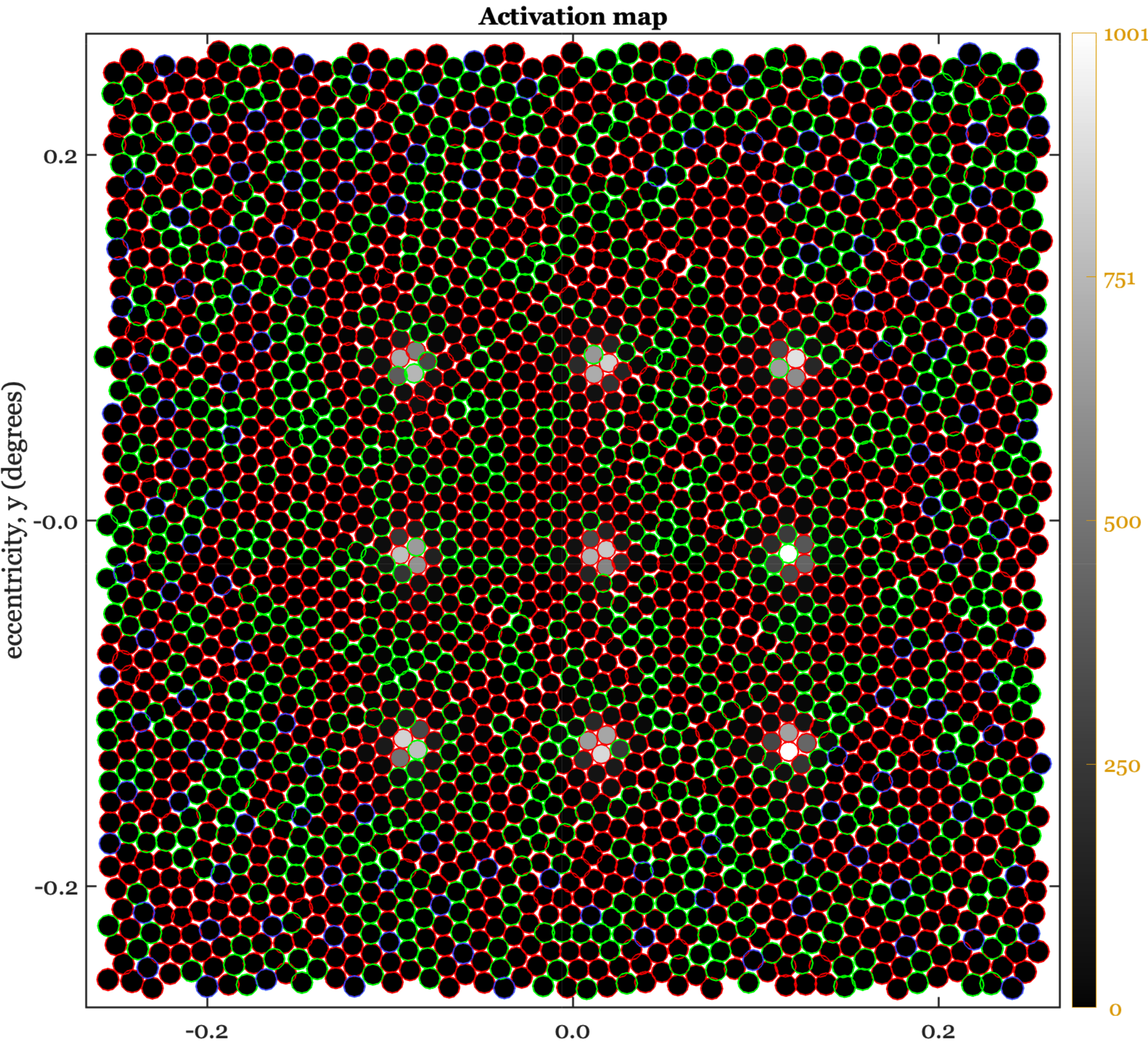
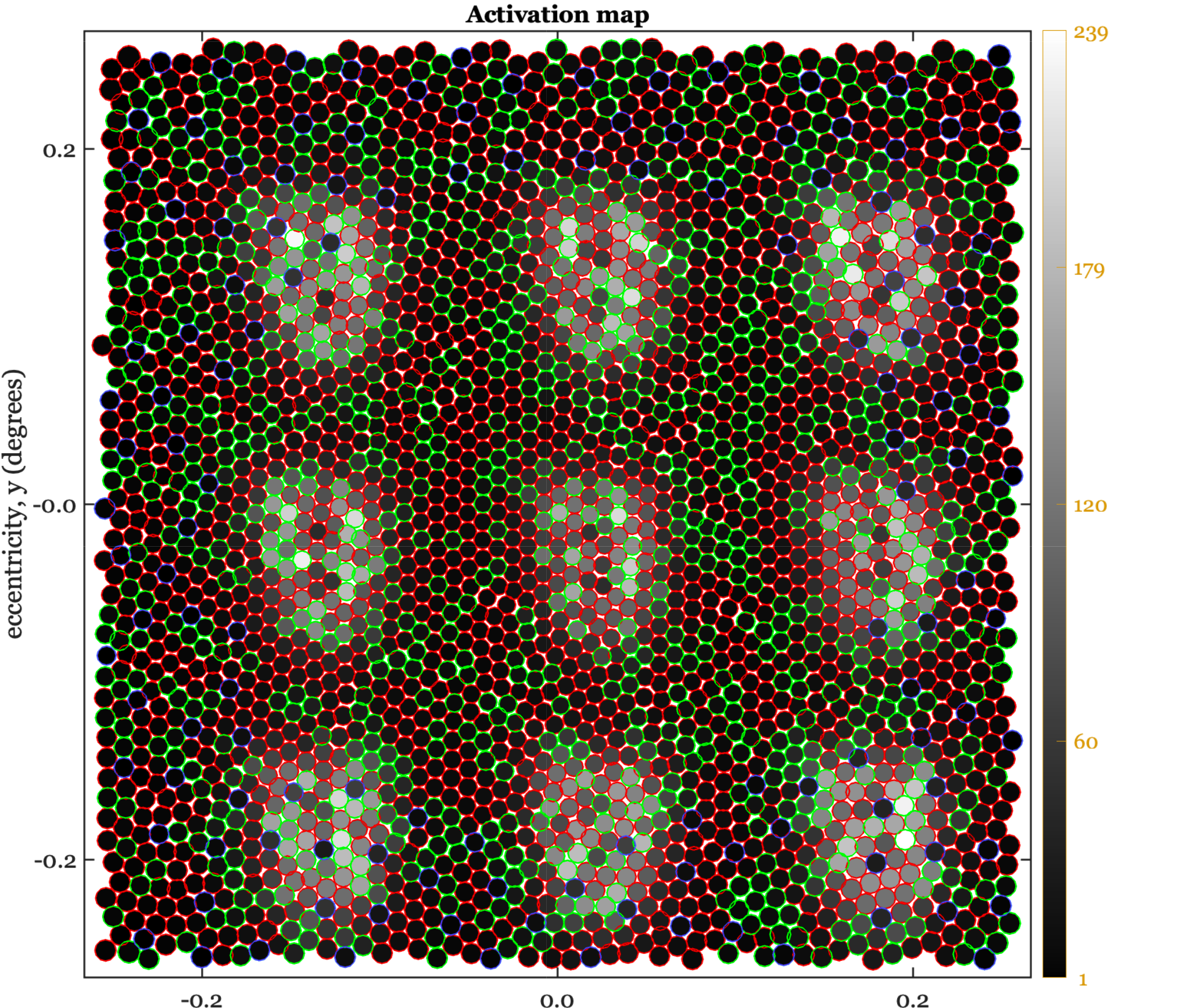
The set of images in this panel illustrates the PSF on the cone mosaic for locations in the central fovea, 3 deg, 6 deg and 12 deg. The original scene is a set of 9 points (3 x 3), spanning about half a degree. The points are broadband lights. In the fovea, the PSF excites about 3-7 cones. In this region this light causes about 2000 excitations per cone.

In the peripheral locations the cone inner segment apertures are bigger, and the blur is bigger as well. The larger blur matches the increased size of the cone apertures, so once again about 3-7 cones are significantly excited. Further, the cones all absorb about 2000 photons. for this subject, at 12 deg eccentricities, the cone apertures are not quite as well matched. Only 2-4 cones are significantly excited and they each capture about 4000 photons.

(a) Each black circle represents the aperture of a cone inner segment. The hot colormap represents the number of expected excitations from the light. In the fovea region each point excites 3-7 cones significantly above the background level.

If we measure an input-referred spatial resolution, the eye’s sensitivity is considerably reduced with eccentricity. If we think purely in terms of the number of excited cones, the signal is much closer to constant from fovea to periphery. Perhaps this latter measure is the important one for how the nervous system is wired up. I can speculate a little, right? Though I sure would like a better story.

22.8.2 PSF wavelength dependence

In normal viewing, the human eye’s optics brings the middle wavelengths are in good focus at the inner segment. Because of chromatic aberration, the short wavelength light is focused at the RGC layer, and measured at the inner segment layer the short wavelength light is considerably spread out (Figure 22.11). The defocus of the short wavelength light is wired into the design of the cone sampling density.

We can see this by comparing the spacing of the L- and M-cones with the S-cone (Figure 22.11). That figure shows the sampling density of the L,M cones separately from the much lower sampling density of the S-cones. There are about 3-5 cones within the point spread of the middle wavelength light, and there are also about 3-5 S-cones within the point spread of the short-wavelength light. Nature has evolved a photoreceptor mosaic so that the spatial sampling of each cone type matches the wavelength-dependent optical blur.

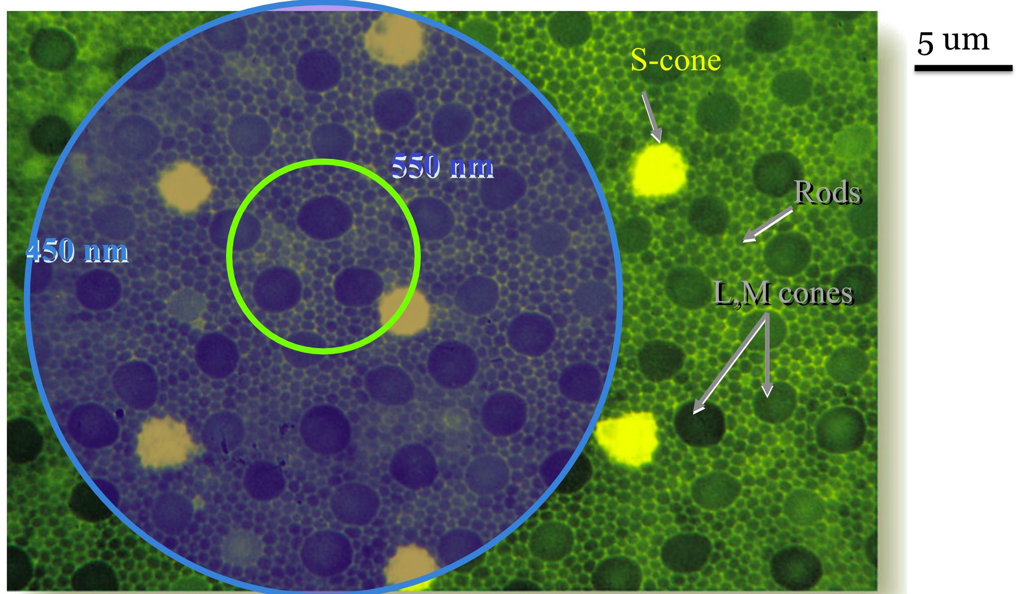
Modern measurements of the eye’s wavefront aberrations enable us to simulate the wavelength-dependent PSF at the cone mosaic effect. Recall that in the very center of the fovea, there are no S-cones. But there are some about 0.2 deg in the periphery. If you click on the images in Figure 22.12, you will see a simulation of the absorptions along with a label of the cone type by the color of the circle around each cone. For the 550 nm light in the left panel, the excitations are spread over only about 3 cones.

For the 450 nm light in the right panel, the PSF is spread over a larger retinal region. But again, click on the image to see it enlarged in a new tab. The number of S-cones excited by the short-wavelength PSF is still only 3-5, as in Figure 22.11. The number of excitations of all the cones, including the S-cones, is much lower for the short-wavelength light. Recall that the short-wavelength light is absorbed by the cornea, lens, and macular pigment. To equate the number of absorptions, we would need to scale the intensity of the light quite a bit.

22.9 Spatial sensitivity in the transform domain

The usefulness of the analyses in the transform domain, in engineering generally and optics specifically, led vision scientists to ask whether measurements using harmonics could be useful for understanding and characterizing the human visual system. Perhaps the first person to see the potential application was the image systems engineer Otto Schade. This is the person who developed the concept of the modulation transfer function (MTF) for image systems engineering questions (Section 12.4.2).

I created four Google docs with historical information about CSF measurements, how to download the historical data, and how to imlement the modern models of the historical and more modern data. Integrate those pages here and write some Matlab scripts to create figures.

Show the data he collected of the CSF (1/MTF) he measured that I include in FOV. Maybe in the human spatial encoding chapter.

The use of harmonics to probe the visual system is quite different from their use in studying typical systems. At many points in this volume I have pointed out that harmonics are particularly valuable stimuli for space-invariant linear systems Chapter 31. These systems have an input and an output. THe use of harmonic stimuli in human vision faces two significant limitations. First, as we have just seen, the system is not at all space-invariant (Figure 22.9). It is justifiable to use harmonics as special stimuli over small regions of the retina, which can be close to space-invariant. Stimuli that span more than a degree or two will not have the special property (harmonics being nearly eigenfunctions) that make them so useful in systems analysis.

Second, even at the earliest stages of vision the neural encoding is not restricted to a single system.

22.9.1 Contrast sensitivity functions (CSF)

Optical scientists use both the space domain (PSF) and the transform domain (MTF) to study their system, and vision scientists use both domains as well. The nonuniformity of the optical blur, coupled with the nonuniformity of the cone spatial sampling, imply that shift-invariant methods only make sense over patches of the visual field. As a result, the carefully controlled harmonics used in vision experiments are modulated over relatively small regions of space.

There are several ways in which this modulation is accomplished in experiments, though perhaps the most common is to use a Gabor function; named after Denis Gabor, the Nobel Laureate credited with the discovery of the laser.

\[ \begin{aligned} g(x,y) &= \exp\!\left( -\frac{(x - x_0)^2 + (y - y_0)^2}{2\sigma^2} \right) [1 + a \cos\!\big(2\pi f x + \phi\big)] \end{aligned} \tag{22.1}\]

Gabor functions are harmonics modulated by a Gaussian. The standard deviation of the Gaussian (\(\sigma\)) controls the spatial spread; the frequency of the harmonic \(f\), controls the center frequency of the image. The phase term, \(\phi\), controls the spatial relationship between the harmonic and the peak of the Gaussian. The central position in the visual field is \((x_0,y_0)\), and the amplitude of the harmonic is controlled by \(a\).

Figure: Show images of different Gabors.

Show classic contrast sensitivity functions (CSF) measured with Gabor patches shown here.

Note: Should we adjust \(f\) and \(\sigma\) together, or should we fix \(\sigma\) and adjust \(f\) on its own. Thinking about the space-variant part of the human visual system, we realize both are important parameters.

22.9.2 Vernier acuity

Gerald and Suzanne lead.

Pierre Vernier

https://www.fisicanet.com.ar/biografias/cientificos/v/vernier-pierre.php

Something about Vernier calipers and the story of Pierre Vernier.

Historical

https://en.wikisource.org/wiki/1911_Encyclop%C3%A6dia_Britannica/Vernier,_Pierre

22.10 TODO

Not sure the astronomy one should be here. Shack-Hartmann should, I think.

Astronomy and adaptive optics

https://en.wikipedia.org/wiki/Pierre_Vernier

fisicanet.com.ar/biografias/cientificos/v/vernier-pierre.php

22.10.1 Ground-based telescopes

quatThese same technologies can be used to look inward, within the eye, rather than outward toward the stars. Realizing this was a very important insight that continues to lead to important insights about the peripheral human visual system (Section 21.1).

Where should the adaptive optics measurement method be? Here or FOV? Adaptive optics measurements of wavefront aberrations, expressed as point spread functions. Thibos and Artal data.

The ability to measure certain properties of the optics was revolutionized by adpative optics - a method that makes real time measurements of the wavefront aberrations of the physiological optics using a Shack-Hartmann wavefront sensor. Just the measurement of the aberrations alone is useful. In addition, it has proben possible to engineer systems that correct for these aberrations in real time, and thus visualize the apertures of the photoreceptors (1-5 \(\mu \text{m}\) diameter) cells in the retina. Further, using video tracking of the eye movements it has proven possible to deliver stimuli to specific, targeted photoreceptors.

First order approximations of the human optics. Simulations with ISETBio of maybe the Westheimer or Ijspeert functions. Eye models?

:::