5 Spectral regularities – Foundations of Image Systems Engineering

5.1 Spectral regularities overview

5.2 Solar Radiation

The Sun serves as Earth’s primary radiation source. The radiation emitted from the Sun’s surface in the visible spectrum remains relatively consistent over time. Due to its significance for imaging and human vision, skylight became an early subject of scientific investigation.

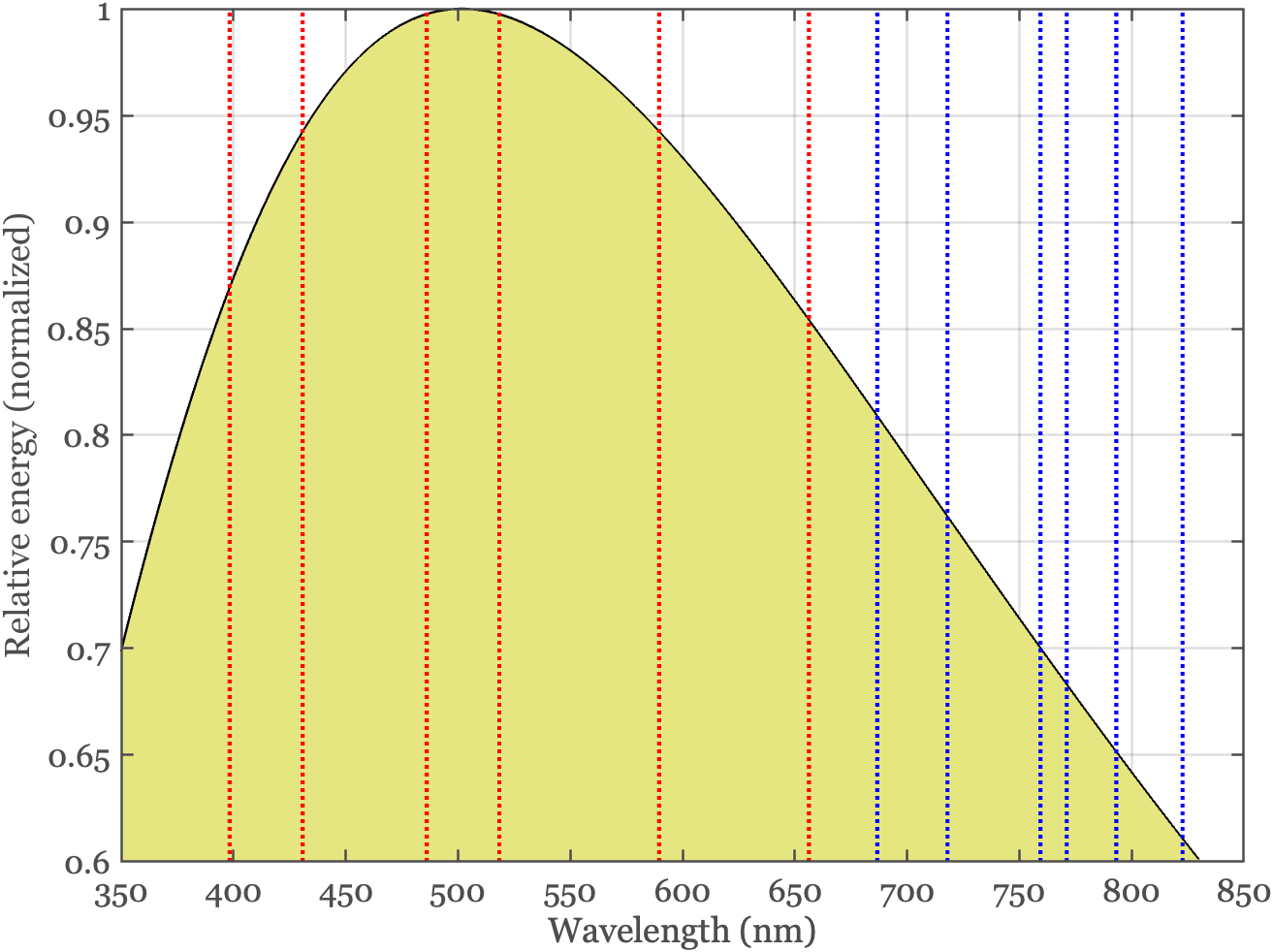
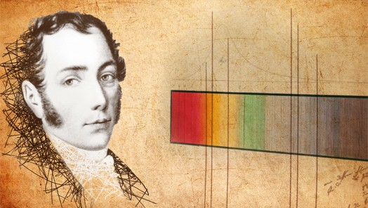
In 1814, Joseph Fraunhofer observed and carefully documented numerous dark lines in the solar spectrum, now known as Fraunhofer lines. It was subsequently discovered that these lines are present because light generated in the Sun’s hot, dense interior (photosphere) travels through its cooler outer layers (chromosphere and corona). During this passage, atoms and ions absorb specific wavelengths of light that correspond precisely to their electron transitions. The reliability of these solar absorption lines allows scientists to use them as reference points to calibrate laboratory instruments for spectral measurements. For example, James Clerk Maxwell used these lines to calibrate the first experimental rig for human color-matching (Maxwell (1860),Maxwell and Zaidi (1993)).

Figure 5.1: The black curve displays the relative solar spectrum, which is stable over time. The red lines indicate are drawn at wavelengths where the spectrum exhibits narrow intensity reductions, known as Fraunhofer lines, that originate from ions and atoms in the Sun’s outer layers. The blue dotted lines mark intensity reductions caused by atmospheric water vapor.

Fraunhofer

Joseph Fraunhofer (1787-1826) was a brilliant applied researcher who worked on the physical properties of materials, particularly glass. He also made important contributions to the theory of image formation and optics.

The Fraunhofer lines, which he discovered while building a device to measure the spectral transmissivity of glass, are reported in a paper reviewing the properties of glass. The relative intensity of these lines are determined by the material composition of the stars, and these measurements are still used in astronomy to determine the composition of celestial bodies. Fraunhofer died at the age of 39, poisoned by heavy metal vapors used in his material research. Europe’s largest body for the advancement of applied research, the Fraunhofer Society, is named to honor him.

This is a good historical review of the Fraunhofer lines and subsequent work.

5.3 Atmospheric Effects

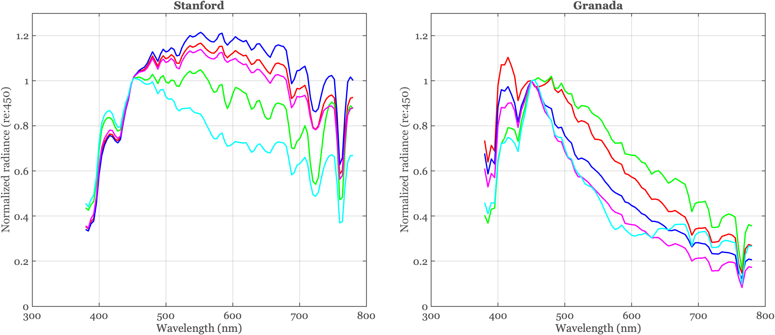
Some of the spectral absorption lines observed at Earth’s surface originate from a different source: water vapor (H₂O) and other molecules in Earth’s atmosphere. Unlike the stable solar absorption lines, these atmospheric absorptions fluctuate relatively quickly with changing weather conditions. There is also atmospheric variation in the skylight spectral power with the time of day, as the radiation’s path length through the atmosphere varies. Longer path lengths — such as during sunrise or sunset — modify the spectral composition of radiation reaching Earth’s surface.

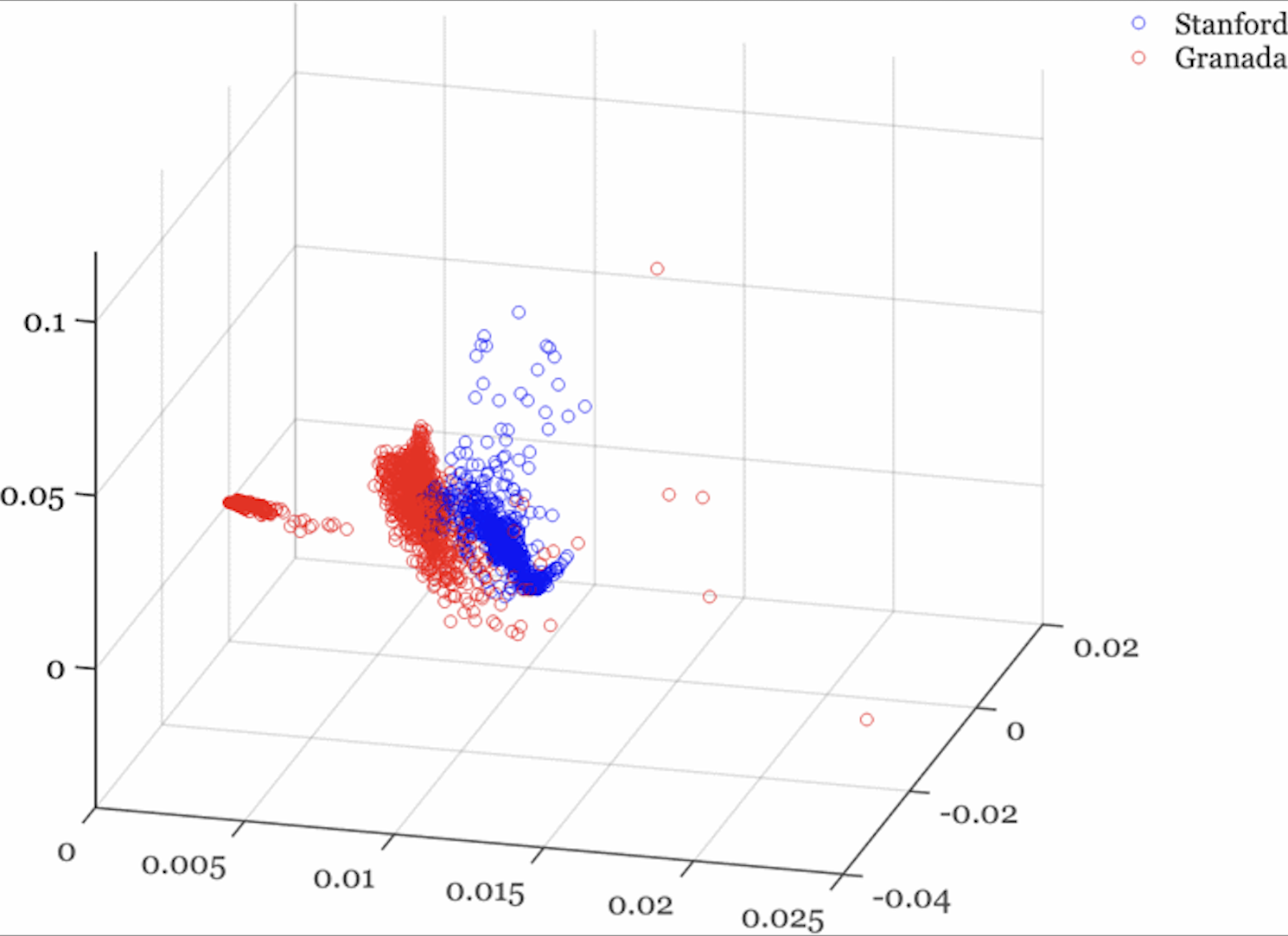
A number of different groups have reported measurements of solar radiation at the Earth’s surface at varying times of day and weather conditions (Judd et al. 1964). Figure Figure 5.2 shows examples of typical variation in the shape of the spectral power distribution in Granada, Spain (Hernández-Andrés et al. 2001) and Stanford, California (DiCarlo and Wandell 2000).

Figure 5.2: The spectral power distribution of daylights sampled at the Earth’s surface in Stanford, California (left) and Granada, Spain (right) at different times of day and weather conditions. The spectra have been scaled to be equal at 450 nm. The curves have different slopes, and their shapes vary with weather and time-of-day. Identifiable Fraunhofer lines and water vapor lines are present in both sets of measurements. The regularities in daylights measured across the Earth’s surface are captured by a CIE standard.

These combined factors—atmospheric composition and path length variations—create a complex, but restricted, distribution of sky radiances at the Earth’s surface. To summarize the regularities, scientists and engineers have created linear models that can represent the natural variations. The original model was introduced by Judd, Macadam and Wyszecki (Judd et al. 1964). They analyzed skylight at the Earth’s surface using about 650 different measurements. They found that the spectral power distributions, normalized to remove absolute radiance level, could be modeled as the weighted sum of three terms: a mean and two basis functions (Figure 5.3). Such a model is useful because it enables us to represent any particular sample using just three numbers, the two weights and an overall scalar to match the level. The model is also useful for applications in which a scene is acquired under full sky illumination, and we would like to estimate the spectral power distribution of the skylight. We only need to estimate the weights, and from those we can make a good estimate of the full spectrum.

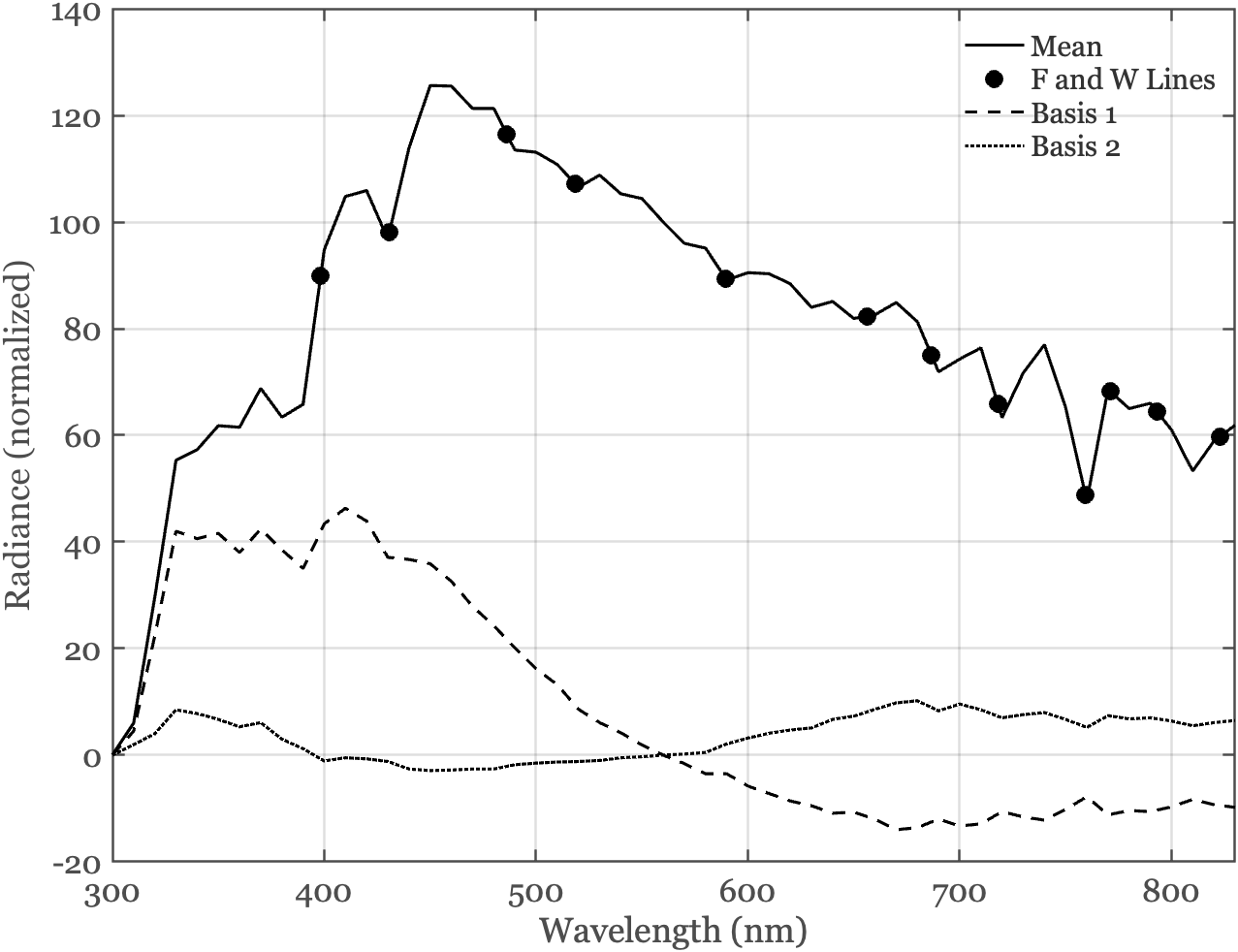
Figure 5.3: The solid curve shows the mean daylight spectrum measured by Judd, Macadam and Wyszecki Judd et al. (1964). Their measurements evolved into a CIE standard linear model for daylights across the Earth’s surface. The solid circles are placed at the wavelengths of Fraunhofer and atmospheric water vapor lines. The dotted and dashed curves are basis functions. Together with the mean, these three curves are a linear model of daylight spectral power distributions.

Do it yourself daylight spectra

When he was a student at Stanford, Jeff DiCarlo decided to measure the daylight outside his office for himself (DiCarlo and Wandell 2000). Checking things for himself is in his nature. Jeff pointed a spectral radiometer at a calibrated surface outside his window and configured a computer to make about ten thousand measurements, one a minute, during the course of a few rainy weeks in California (January 28, 2000 to February 16, 2000). I included a sample of 1000 of these measurements in ISETCam, and I have the whole group along with time stamps if you want them.

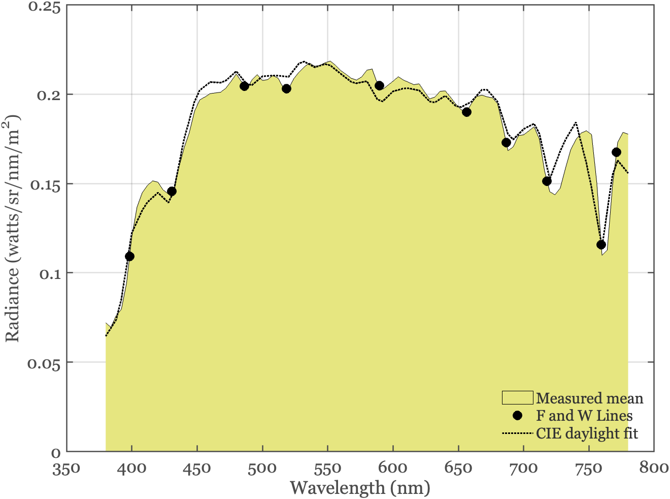
Figure 5.4: Average daylight measurements on the Stanford campus (solid) and CIE daylight basis fit to the measured average (dotted). The solid circles are placed at the locations of Fraunhofer and water vapor wavelengths.

Figure 5.4 shows the mean spectral power distribution of these measurements. You can see that the instrument recorded several ‘notches’ in the spectrum at wavelengths corresponding to the Fraunhofer and water vapor lines. We also asked whether these data could be fit by the CIE linear model - and the least-squares fit is shown by the dotted line. I suspect there is an instrument calibration error of a few nanometers at wavelengths above 700nm, and were I to write a research paper based on these data, I would probably introduce the correction because I believe the physics on the locations of these wavelengths is secure. This analysis might provide you with a sense of the relative accuracy of measuring and approximating spectra with conventional lab equipment.

The regularities in the sky radiance are even more constrained than the linear model. First, the weights are correlated: When you know one of the weights, you can make a reasonable guess about the other weight. Also, some weights are impossible because they would produce negative values in the spectrum DiCarlo and Wandell (2000). Thus, the linear model gets us part of the way to establishing the regularities, but there is even more to be measured.

Daylight weights

5.3.1 Correlated weights

Figure 5.5: (PDF Snapshot): The daylight basis weights from the Granada and Stanford data sets. The weights are clustered within a plane, although there are occasional outliers. The orthogonality of the basis functions does not imply independence or orthogonality of the measured basis weights.

5.4 Surface spectral reflectance regularities

Vision enables us to interpret the environment by recording the how the ambient illumination interacts with things (e.g., objects) and stuff (e.g., water). Four things can happen when electromagnetic radiation interacts with a surface. The radiation arriving at a surface might be (a) reflected, (b) absorbed, (c) pass through, or (d) interact with the material and generate new radiation (fluorescence). We will consider each of these interactions in different sections of this book. Here, we describe some regularities how light is reflected from many common materials.

Things and Stuff

I am fond of a distinction that Ted Adelson introduced to help think about the environment: “things and stuff” Adelson (2001). Things are the countable, discrete objects with defined shapes and boundaries (e.g., cars, chairs, animals). Stuff is amorphous materials or textures without fixed boundaries (e.g., water, grass, sky, sand). Dividing the environment into these categories also helps us set computational goals.

The distinction helps separate out the types of algorithms we might apply to understand the environment. Segmentation applies to things which are analyzed for object identity and function; in contrast, stuff is regionally based on texture and material properties. A great deal of computer vision focuses on tasks such as naming or counting cars on the road, people in the room, airplanes in the sky. We wish to be able to recognize such things whatever their material might be. A vision system must also be able to make judgments about a sandy beach, a cloudy sky, a grassy hillside. We wish to be able to recognize such stuff whatever its shape might be.

A related challenge in human vision is quantifying the appearance of things and stuff, and for this challenge surface reflectance, texture, and context (e.g., ambient illumination, or what things and stuff are nearby) all play a role Schmid et al. (2023). A corresponding concept - something we might call appearance for a computer vision system - seems desirable. One way to formulate the problem of appearance for a computer vision system is to use and estimate of material reflectance and texture to mean appearance for the computer.

The COCO-Stuff 164k dataset has many images categorized in terms of ‘things’ and stuff.

The radiation incident on a small, planar patch of material can come from different directions, which we can specify by two angles. The intensity of the reflected radiation will also vary with direction (two more dimensions). The incident and reflected light can be measured as the intensity for different wavelengths and polarizations (two more dimensions). We will set aside fluorescence for the present, returning to it later. Hence, a full description of surface spectral reflectance requires specifying multiple parameters.

Despite this potential complexity, there are many relatively simple cases that are simpler to describe and still useful. We will work our way up from the simplest case to increasingly complex descriptions, identifying regularities along the way.

5.5 Diffuse reflectance

An important type of reflectance, diffuse reflectance, or Lambertian reflectance. The incident light is reflected with roughly equal intensity in all directions within the hemisphere above the surface. This occurs when the surface is rough at a microscopic level, comprising many little facets. When the incident light arrives, it will be reflected by one of the facets which are oriented equally in all different directions. Importantly, not all of the incident light is scattered; some of it is absorbed. The fraction that is absorbed varies with wavelength. The fraction that is scattered is called the diffuse spectral reflectance function.

Many objects, like paper, clothing, and walls, are mainly diffuse reflectors, and the spectral reflectance function is a dominant factor in how we perceive surface color. You can judge to what extent a material is a diffuse reflectance by viewing it from different positions, say by moving your head or walking around the room. For diffuse materials the reflected light will be about the same. Other materials, such as the highlights reflected from a car, vary in intensity and color appearance as you move around, appearing bright from some positions but not others. Such materials are not diffuse.

Johan Lambert

The term Lambertian surface honors the Swiss physicist, Johann Lambert (1728-1777) who formalized the mathematical description. Many surfaces are modeled as Lambertian in computer graphics, or assumed to be Lambertian in computer vision estimates of the environment. Examples of materials with Lambertian reflectance include chalk, plaster, uncoated paper, and matte paints made from pigments.

Adding additional details about the surface reflectance can improve the system performance, but it is common to start with a Lambertian approximation.

Figure 5.7: Johann Lambert. His ideas were spread widely.

Lambert worked on many topics concerning geometric optics, and he contributed an important book Photometria that incorporated many important geometric ideas, explaining the relative brightness of objects as seen from different points of view. Using his excellent mathematics, and the assumption that light travels in straight lines, he showed that illumination is - proportional to the strength of the source, - inversely proportional to - the square of the distance of the illuminated surface, and - the sine of the angle of inclination of the light’s direction to that of the surface. He also wrote a classic work on perspective and contributed to geometrical optics.

I was interested to learn that Lambert was the first to show that \(\pi\) is an irrational number, a claim that the great Euler sought to prove as well.

Figure 5.8: Sample spectral reflectance functions of clothing. The fraction of reflected light, wavelength-by-wavelength, is between 0 and 1. Such smooth spectral reflectance curves are typical of many surfaces. Surfaces that are not diffuse can be modeled as having a diffuse component with a smooth spectral reflectance.

We can summarize the spectral reflectance of a diffuse material relatively simply because we do not need to specify the input and output angles. We only need to measure the fraction of incident light, for each wavelength, is reflected. This is called the spectral reflectance function. In the visible band these functions are often smooth, and it is possible to summarize them using only a few parameters. It is not realistic to sample all possible surfaces, but we can consider surfaces in a particular context (e.g, walking in a forest, clothing, the interior of a commercial office building, driving on a highway, or medical images of the body). The likely surfaces in any particular context can be usefully summarized with a linear model Hardeberg (2002). The number of basis functions needed will depend on the task requirements (e.g., 5% or 1% accuracy). But the general usefulness of a linear model approximation as a computational tool is not in doubt.

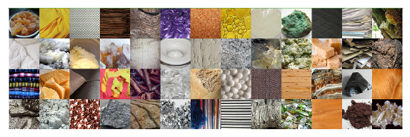
Over the decades a number of imaging groups have measured the reflectance of many types of materials, including paints, minerals, plants, clothing, and various biological specimen such as skin and teeth. Government agencies, particularly those involved in remote sensing, have measured the reflectance of many materials that might be seen in satellite images. As a general rule, the spectral reflectances of the samples reported in the literature are approximated to an accuracy of a few percent by linear models using between 3 and 8 basis functions.

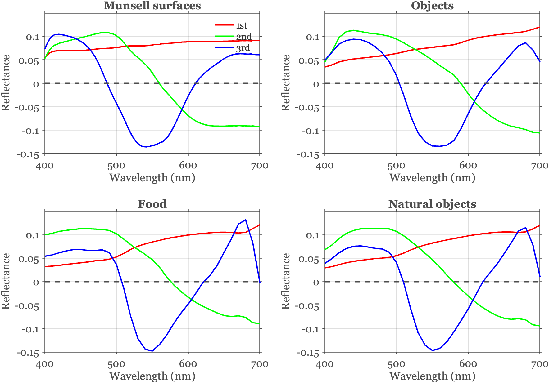
A Finnish group, for example, measured 1269 different color swatches from the Munsell Book of Colors. This widely used book spans a wide range of color samples that provides designers with a method for identifying, selecting, matching, and communicating about color. Parkkinen et al. (1989) made their spectral measurements at 1 nm resolution. A linear model using three basis functions fits all the measurements with an error of about 2.5%. A linear model with 5 basis functions fits the data to within about 1%. This accuracy is usually often enough for image systems applications (Figure 5.9 A).

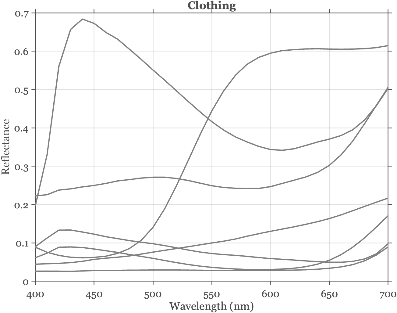
The linear models for diffuse surface reflectance of several types of common materials are similar (Figure 5.9). The data from Vrhel and colleagues Vrhel et al. (1994), included in ISETCam, measures a few dozen surfaces from several different groups (paint, natural objects, man-made objects, food). It is likely the authors chose the samples to have similar means and a broad representation of color appearances. For this sampling strategy, the first component will necessarily be similar. But the 2nd and 3rd basis functions are also similar, and this is less likely to be a selection artifact. Rather, the similarity arises because the diffuse spectral reflectance functions are very smooth functions wavelength Maloney (1986).

Figure 5.9: Three basis functions comparing the basis functions derived from the Parkkinen et al. (1989) Munsell Color Book data (upper left) and three different categories of materials. The basis functions are not identical, but they have many similarities, including the wavelengths of the zero-crossings of the 2nd and 3rd basis functions. Data from Vrhel et al. (1994) and distributed in ISETCam.

5.6 Specular reflection (mirror)

The conceptual opposite of diffuse reflection is mirror reflection. In this case, an incident light ray from one direction reflects from the surface in just one direction. The geometry of mirror reflection is shown in Figure 5.10. The incident ray, reflected ray, and surface normal all lie in the same plane (the plane of incidence). The angle of incidence is equal to the angle of reflection, and the surface normal acts as a line of symmetry in the plane of incidence.

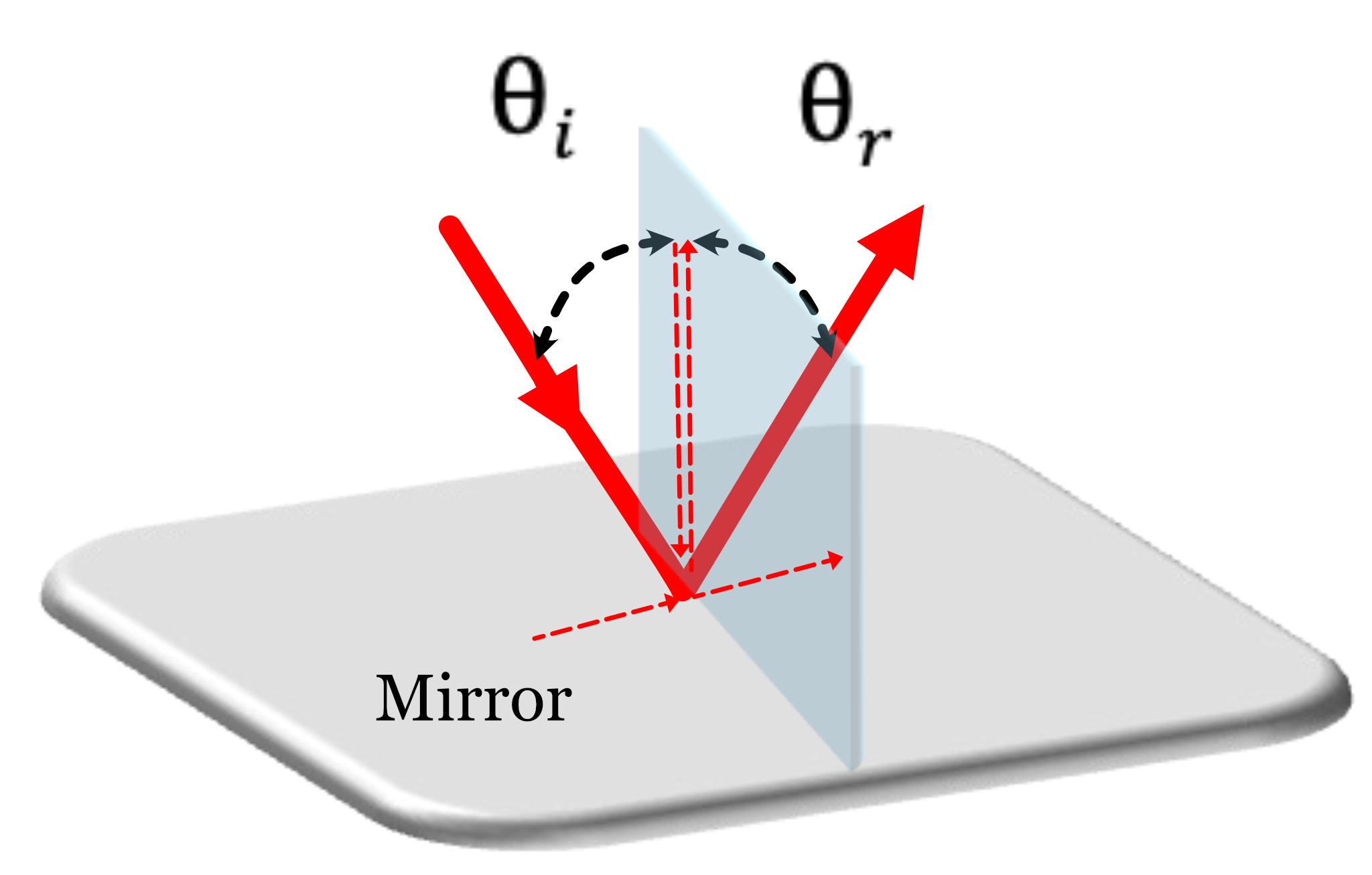
Figure 5.10: Geometry of mirror reflection. The incident and reflected rays have a component parallel to the surface normal and a component in the surface plane. The component in the surface plane remains the same after reflection; but the component in parallel to the surface normal is points in the opposite direction (sign-reversed (). The absolute value of the ray angles with respect to the surface normal of the two rays is matched, \(\theta_i\) = \(\theta_r\).

It is useful to consider vector components of the incident and reflected ray separately. Suppose that the incident light comes from a direction represented by the unit vector \(\mathbf{i}\), and the surface normal vector is \(\mathbf{n}\). The direction of the reflected ray, \(\mathbf{r}\) is calculated this way:

\[ \mathbf{r} = \mathbf{i} − 2 (\mathbf{i} \cdot \mathbf{n}) \mathbf{n} \tag{5.1}\]

The term (\(\mathbf{i} \cdot \mathbf{n}\)) is the projection of the incident ray onto the normal ray. We subtract twice that amount from the incident ray, which flips this component. The component of the incident and reflected rays that is parallel to the surface are the same. The net effect is that the incident and reflected rays form equal angles on opposite sides of the surface normal.

The light reflected at the interface of the surface does not interact with the material. Thus the spectral power distribution of a mirror reflection is approximately equal to the spectral power distribution of the incident radiance.

Common mirrors are close to perfect specular reflectors in the sense that a very small set of collimated rays is reflected over a very small angle of output rays. There are only small deviations from slight surface imperfections. For scientific applications this approximation may not be adequate, and additional steps are taken to polish mirrors, making them increasingly perfect.

Many materials are approximately specular, but not perfectly so. In these materials a narrow bundle of incident rays is reflected mainly in the specular direction, but there is some spread of the reflected rays. Figure 5.11 compares different conditions, including a diffuse reflectance, nearly perfect specular, and mostly specular case.

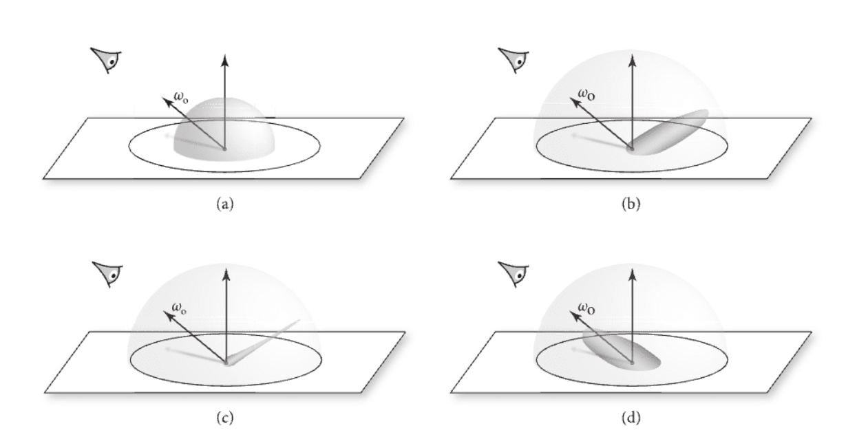
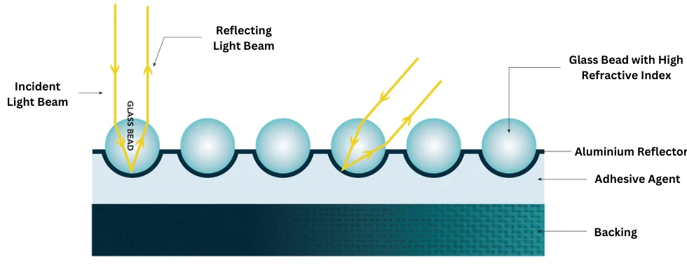
Figure 5.11: Comparisons of (a) diffuse, (b) glossy specular, (c) perfect specular, and (d) retroreflective materials. Figure 9.1 from PBR book. https://www.pbr-book.org/4ed/Reflection_Models

The figure includes a fourth interesting case: retroreflective materials. For these materials the reflected ray is sent back in the same direction as the incident ray. These materials can be created by embedding small, spherical, glass beads with a metallic back surface into the material Figure 5.12. The glass beads refract the incident ray, the metallic surface returns the ray, which is again refracted, so that the net effect is the reflected ray is returned in the direction of the incident ray. Glass beads with a metallic backing are often built into road markings and road signs. Light from a car’s headlight is scattered back towards the driver, increasing the visibility of the road marking or sign during nighttime driving.

Figure 5.12: Glass beads made into a retroreflective material. (Source: roadmarkingsupplies.com, https://roadmarkingsupplies.com/reflective-glass-beads-wholesale-for-road-marking-paints/)

5.7 Dichromatic reflectance model (DRM)

The dichromatic reflectance model (DRM) is another useful surface reflectance model that serves as an approximation for light reflected from inhomogeneous dielectric materials (non-conductors like plastics, paints, wood, skin, etc.). The model approximates reflectance as a weighted sum of a diffuse term and a glossy specular term. This model is used in computer vision applications where the user would like to identify specular reflections.

A fraction of the incident light is reflected at the surface (interface). This light has a mirror-like reflectance that preserves the spectral power distribution and glossy specular spatial distribution. The remaining fraction of the light passes through the interface into the (subsurface) where it interacts with the material’s pigments, both by diffuse scattering and absorption. The subsurface reflectance is usually assumed to be Lambertian, as the subsurface pigments are randomly positioned and oriented. The reflected light, \(C(\lambda)\) is the sum of the interface and subsurface terms

\[ C(\lambda) = m_s(g) I(\lambda) E(\lambda) + m_d(g) D(\lambda) E(\lambda) \tag{5.2}\]

\(E(\lambda)\) is the spectral power distribution of the light; \(D(\lambda)\) is the diffuse subsurface reflectance, which is characteristic of the material. The terms \(m_s(g)\) and \(m_d(g)\) are geometric scaling factors whose values depend on the illumination and viewing angles. These angles are ordinarily represented with respect to the surface normal at the surface point \(g\). The reflected light, \(C(\lambda)\) is sometimes called the color signal because this spectral radiance is an important contributor to the visual system’s color judgment. (Though, I have friends who object to this term). \(I(\lambda)\) is the interface spectral reflectance is often assumed to be constant across wavelengths, which further simplifies the formula

\[ C(\lambda) = m_s(g) E(\lambda) + m_d(g) D(\lambda) E(\lambda) \tag{5.3}\]

The DRM is used in computer vision algorithms such as illuminant estimation, specular highlight identification and removal, and material classification. It is, however, limited because it does not accurately model complex surfaces. Also, it is difficult to apply to scenes with multiple light sources or very large light sources, such as scenes with light sources that span the sky.

DRM Illuminant estimation

Suppose the interface reflectance, \(I(\lambda)\) is approximately constant so that we accept Equation 5.3. If we measure the reflected light from a DRM material at a few angles, we will obtain values that differ because of the geometric terms, \(m_s\) and \(m_d\). These different estimates can be represented as a two-dimensional linear model.

The linear terms we estimate from any single surface, say using principal components, may not be precisely aligned with \(E(\lambda)\) and \(D(\lambda) E(\lambda)\). But if there are two or more different dichromatic reflectance type materials near one another, their linear models must have a shared dimension, \(E(\lambda)\). Thus, we can estimate the principal components of both surfaces, and then find the vector equal to the intersection of these linear models, we will recover the local spectral power distribution of the illuminant.

5.8 Bidrectional reflectance distribution function (BRDF)

The bidirectional reflectance distribution function (BRDF) characterizes how light rays of wavelength \(\lambda\), incident at the surface at an angle \(\omega_i\), are reflected. The reflected, outgoing light is specified at all angles \(\omega_o\). Both \(\omega_i\) and \(\omega_o\) are measured with respect to the surface normal. We can write the intensity as a function of input and output angles as the function \(B(\omega_i,\omega_o,\lambda)\). The reciprocity of principle of light¹ implies that the BRDFs, with only a few exceptions, obey this symmetry relationship.

\[ B(\omega_i,\omega_o,\lambda) = B(\omega_o,\omega_i,\lambda) \tag{5.4}\]

Each of the direction vectors is specified by two parameters, typically defined with respect to the surface normal. One parameter is the angle around the surface normal (azimuth) \(\phi_i, \phi_o\), and the second is the elevation \(\theta_i, \theta_o\) of the ray. We conventionally describe the BRDF with three parameters, but there are really five parameters in there. That makes the BRDF tedious to measure.

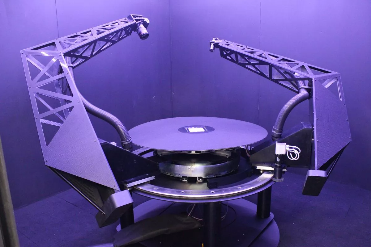
The instrument used to measure the BRDF is called a gonioreflectometer. The instrument has a light source that can be positioned to illuminate the surface at many different angles (typically on a sphere), and a detector that can be positioned at many locations on the sphere. There are many different designs for gonioreflectometers. The one in Figure 5.13 shows a surface is placed on a stage that can be rotated. The light and camera are on two arms whose positions can be controlled, sweeping out the possible angles for the incident and reflected light. To measure the reflectance of a surface requires calibrating the amount of incident light, say by making a measurement with a perfect, white diffusing surface, and then making a second measurement with the material of interest. The ratio of the responses is the reflectance. The same calibration measurement can be re-used for multiple materials of interest.

Figure 5.13: Example of a **gonioreflectometer**. The light source and detector are on robot arms that can be positioned around the surface. If we fix the wavelength and angle of the incident light ray, we can specify the relative intensity of the reflected light as an image that spans the two angle parameters

The input and output angles are 2-vectors and the BRDF is a scalar function. We can make all of the angles explicit this way.

\[ B(\omega_i, \omega_o, \lambda) = f_r(\phi_i,\theta_i,\phi_o,\theta_o,\lambda) \tag{5.5}\]

5.8.1 Theoretical BRDF

Cook Torrance mainly here.

5.8.2 Data driven BRDF

There are papers measuring BRDFs and modeling them using linear models and nonlinear models. Data driven approach.