14 Photons and Electrons
The book is still taking shape, and your feedback is an important part of the process. Suggestions of all kinds are welcome—whether it’s fixing small errors, raising bigger questions, or offering new perspectives. I’ll do my best to respond, but please keep in mind that the text will continue to change significantly over the next two years.
You can share comments through GitHub Issues.
Feel free to open a new issue or join an existing discussion. To make feedback easier to address, please point to the section you have in mind—by section number or a short snippet of text. Adding a label characterizing your issue would also be helpful.
Last updated: November 2, 2025
14.1 Photons and Electrons overview
The transition from film to digital imaging, enabled by semiconductor technology, has profoundly changed how we record and process images (Boyle and Smith (1970); see Preface). Digital image sensors use arrays of tiny, light-sensitive elements called photodiodes.These are semiconductor devices that convert incoming light into electrical current. Photodiodes are the essential building block of all modern image sensors.
The earliest digital image sensors, known as charge-coupled devices (CCD), were built using metal-oxide semiconductor technology (MOS). Measuring the electrons captured by the array of photodiodes in a CCD requires significant power, making them unsuitable for mobile devices and limiting their early adoption to scientific and other high-end applications.
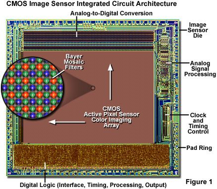
A major breakthrough came with Eric Fossum’s invention of the Complementary Metal-Oxide Semiconductor (CMOS) image sensor (Fossum (1993); Fossum et al. (1995)). By implementing an active pixel sensor (APS) circuit in CMOS, Fossum enabled image sensors to be manufactured using mainstream microelectronics processes. This dramatically reduced power consumption and allowed integration of light-sensing pixels with timing, control, and signal processing circuitry on the same chip (Figure 14.1). These advances paved the way for the widespread adoption of electronic image sensors in mobile devices and many other applications.
14.2 Photoelectric effect
The physical principle underlying photodiode operation—converting light into electrons—is called the photoelectric effect. Understanding how materials convert light into electrical signals is a foundational chapter in physics and engineering, shaped by experiments and theories that changed how we think about light and matter. In metals and vacuum tubes, the effect refers to electrons being emitted from a surface into vacuum. In semiconductors (as in photodiodes), absorbed photons create mobile charge carriers (electron–hole pairs) that are collected by circuitry.
Heinrich Hertz was the first to report an unexpected phenomenon related to electromagnetic waves that would later be recognized as the photoelectric effect (Hertz 1887a, b). His primary goal was to measure the electromagnetic waves predicted by Maxwell’s theory. For this, he used a two-part apparatus:
The Transmitter: This consisted of a large induction coil connected to a spark gap (often with attached metal plates acting as a dipole antenna). The induction coil produced high-voltage pulses, causing powerful, oscillating sparks to jump across this gap. These sparks were the source of the electromagnetic radiation (radio waves) that Hertz aimed to study.
The Receiver: This was a separate, much smaller loop of wire, also containing a small spark gap. The receiver was placed at a distance from the transmitter. When the electromagnetic waves from the transmitter propagated to the receiver, they induced an oscillating current in the receiver loop. If the induced current was strong enough, a tiny spark would jump across the receiver’s gap, signaling the detection of the electromagnetic waves.
During these experiments Hertz made a crucial incidental observation: a spark in the receiver gap was significantly enhanced—jumping a longer distance—when the gap was illuminated by ultraviolet (UV) light from the transmitter’s spark. Placing a glass plate (which blocks UV) between the transmitter and receiver diminished the receiver spark; a quartz plate (which transmits UV) did not. Hertz concluded that UV light was facilitating the spark in the receiver gap. This was the first report of what we now call the photoelectric effect: light causing emission of charged particles (later identified as electrons) from a material surface, thereby influencing electrical signals.
Hertz correctly concluded that UV light was somehow facilitating the spark in the receiver gap. This observation was the first report of the photoelectric effect – the phenomenon where electromagnetic radiation, specifically UV light in this case, causes the emission of charged particles (later identified as electrons) from a material surface, thereby influencing electrical signals. The central challenge of the photoelectric effect is to model how electromagnetic radiation—light—interacts with a material to generate an electrical signal.
14.3 Discovery of the photon
In 1897, J. J. Thomson conclusively demonstrated that cathode rays are streams of negatively charged particles—electrons—with a specific mass and charge, much smaller than an atom.
In 1902, armed with knowledge of electrons, Philipp Lenard carried out a series of important experiments. He observed that increasing the intensity of the incident light increased the number of emitted electrons but did not increase their kinetic energy. Instead, the energy of the emitted electrons depended on the wavelength of the light: shorter wavelengths (higher frequencies) produced more energetic electrons. Lenard also identified a threshold wavelength—if the light’s wavelength was too long (i.e., its frequency too low), no electrons were emitted, regardless of how intense the light was. These results posed a serious challenge to classical wave theory, which predicted that energy should increase smoothly with intensity, not depend on frequency.
The Experimental Setup
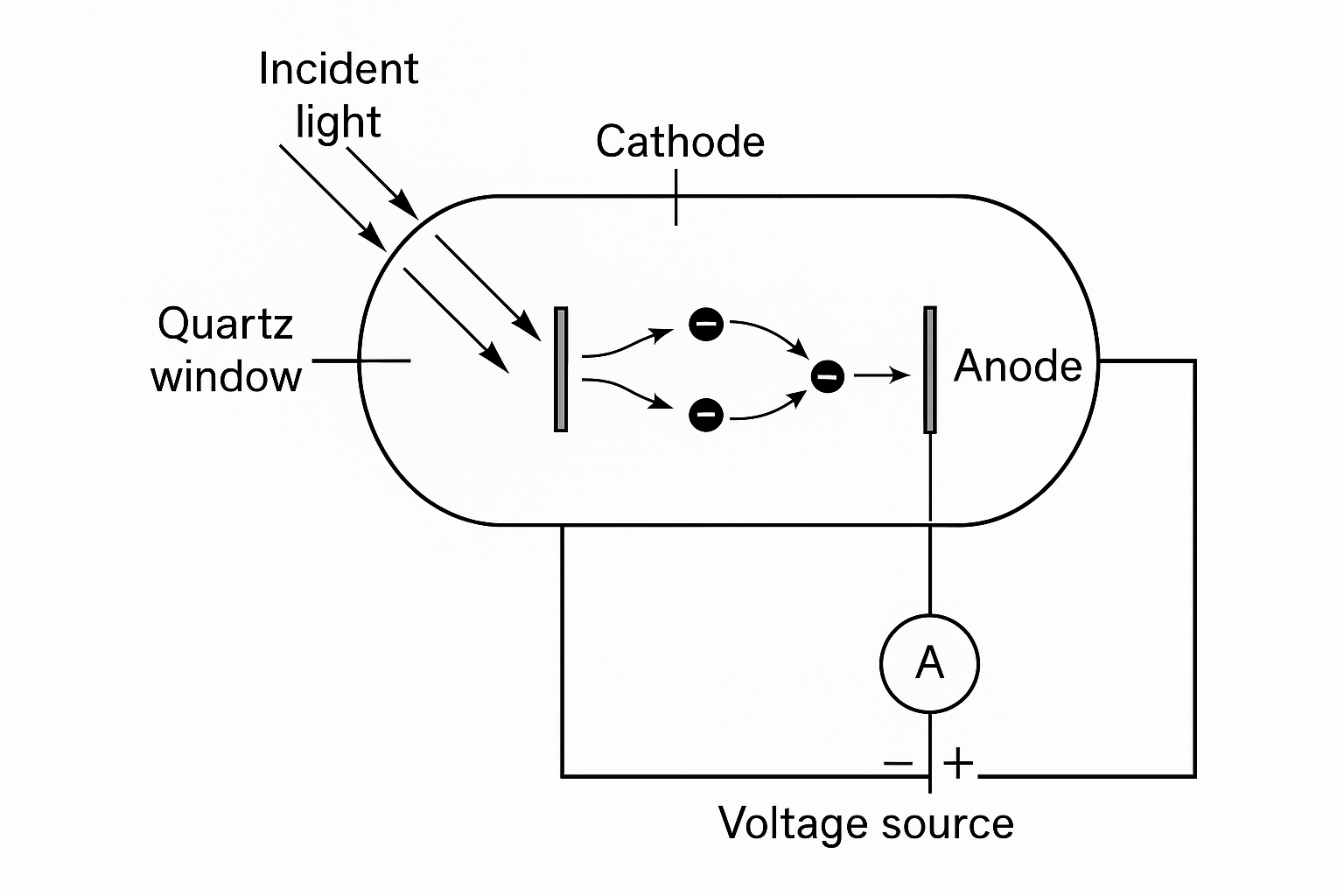
Philipp Lenard refined the early photoelectric experiments of Hertz by introducing a carefully controlled photoelectric tube. The apparatus consisted of two metal electrodes—a cathode and an anode—sealed within a glass envelope that provided a near-vacuum. The key components were:
- Cathode: a clean metal plate (often zinc or platinum) serving as the illuminated surface.
- Quartz window: allowed ultraviolet light to enter the tube without absorption.
- Anode: a collecting electrode positioned to receive emitted electrons.
- Adjustable voltage: an adjustable potential difference between the cathode and anode.
- Electrometer: a sensitive measuring device to record the resulting current (not shown).
When he illuminated the metal cathode, electrons were produced (the photoelectric effect) and ejected into the vacuum. They were collected by the anode. The rig could both apply a voltage between the anode and cathode as well as measure the current. In the experiments he measured how the current changed as light was presented and the potential difference was varied. He found that the photoelectric current reached a saturation level when all emitted electrons were collected, and it dropped to zero when the applied voltage was sufficiently negative to repel even the most energetic electrons.
How the Electron Energy Was Deduced
The crucial measurement in Lenard’s experiment was the stopping potential, \(V_s\), the retarding voltage required to reduce the photoelectric current to zero. This provided a direct measure of the maximum kinetic energy of the emitted electrons:
\[ e V_s = \tfrac{1}{2} m v_{\text{max}}^2 \]
where \(e\) is the electron charge and \(v_{\text{max}}\) is the velocity of the fastest emitted electrons.
By systematically changing the light intensity and wavelength, Lenard discovered two key laws:
- Increasing intensity (at fixed wavelength) increased the number of emitted electrons, and thus the measured current, but did not change the stopping potential (\(V_s\)).
- Increasing frequency (decreasing wavelength) increased the stopping potential—hence, the energy of the electrons.
These findings showed that the energy of photoelectrons depends on the frequency of the incident light, not its intensity—a result that could not be explained by classical wave theory.
Einstein’s photoelectric equation (1905) explains Lenard’s observations: \[ e V_s = h \nu - \phi, \]
where \(h\) is Planck’s constant, \(\nu\) is the light frequency, and \(\phi\) is the minimum energy required to emit the electron from a material into a vacuum. It is a surface-dependent material property (typically 2–5 eV for metals). In semiconductors used for photodiodes,this threshold is set by the bandgap, which for silicon is 1.12 eV.
At the same time, physicists were trying to explain the spectrum of light emitted by a blackbody—a perfect absorber and emitter of radiation. In 1900, Max Planck tackled this problem. He found a formula that matched the observed spectrum, but only if he assumed that energy exchange (joules) between matter and radiation occurred in discrete amounts.
\[ E = n h \nu \]
Here, \(n\) is an integer; \(\nu\) is the frequency (\(1/sec\)) of the radiation; and \(h\) is a constant — now called Planck’s constant (\(h = 6.62607015 \times 10^{-34}\) joule-seconds). Planck proposed that the oscillators in the material’s walls could only transfer energies in discrete steps. This quantization explained why the measured absorption and emission of light matched the observed spectrum, even though the light field itself was continuous.
In 1905, Albert Einstein went further. He proposed that we should not think of light as a continuous wave that becomes quantized through an interaction with the material. Rather, he argued, light itself quantized into discrete packets of energy—later called photons. The energy of each photon is proportional to its frequency, and inversely proportional to its wavelength
\[ E = \frac{h c}{\lambda} \tag{14.1}\]
where
- \(h\) = Planck’s constant (\(6.626 \times 10^{-34}\) J·s)
- \(c\) = speed of light in vacuum (\(3.00 \times 10^8\) m/s)
- \(\lambda\) = wavelength (in meters)
This hypothesis went beyond Max Planck’s work, which assumed the quantization was part of the mechanism when radiation interacted with matter. Einstein suggested that light in free space behaves as localized energy quanta, capable of transferring energy to electrons one photon at a time. His theory explained both Planck’s observations and all of Lenard’s experiments. His theory, however, left unexplained the many verifiable findings from Huygens, Fresnel, Maxwell and others concerning the wave nature of electromagnetic radiation. Even so, the photoelectric theory laid the groundwork for the next generation’s work in quantum physics that was needed to resolve these differences.
14.4 Wave-particle duality
For much of the 19th century, Newton’s idea that light was made of tiny particles (corpuscles) was set aside, as experiments overwhelmingly supported the wave theory of light—interference and diffraction patterns provided strong evidence for wave-like behavior. However, the photoelectric effect presented results that could not be explained by wave theory alone, forcing physicists to recognize that light sometimes behaves as a particle as well. This is the essence of the wave-particle duality.
Einstein did not ignore the wave phenomena. For much of his career, he worked towards a new set of principles that might be called a “statistical wave-particle” model, in which photons retain a wave-like “guiding field” or statistical distribution that determines their path. He imagined that individual photons are particles, but their collective behavior is governed by an emergent, wave-like probability distributions that creates the familiar diffraction patterns.
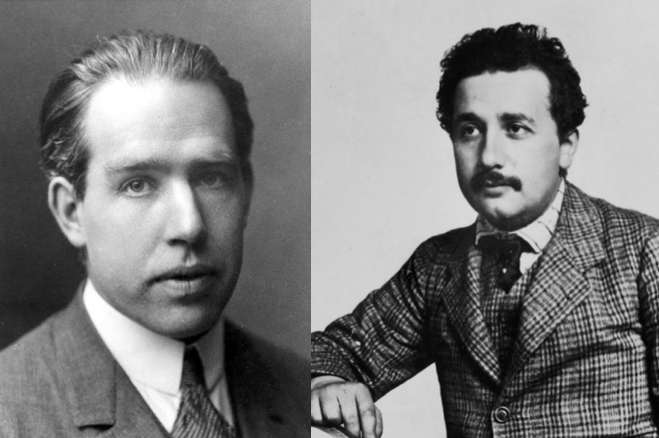
A different, revolutionary theory sprung forth from the next generation, including Neils Bohr. This theory, quantum mechanics describes electromagnetic radiation by a mathematical object called the wavefunction, which provides the probabilities of different outcomes. When experiments are designed to reveal wave-like effects (such as interference), light behaves as a wave. When experiments probe particle-like effects (such as the photoelectric effect), light behaves as a particle.
The young theorists argued that both descriptions are necessary, and neither alone is sufficient to fully describe the nature of light. Einstein was reluctant to accept this framing calling it implausible; Bohr argued that Einstein was clinging to classical intuitions about reality that quantum mechanics had shown to be inadequate. From Bohr’s perspective, the probabilistic nature of quantum mechanics wasn’t a sign of incomplete knowledge - it was a fundamental feature of nature at the microscopic scale. Bohr believed that concepts like “determinism” and “objective reality independent of observation” were classical prejudices that had to be abandoned. He argued that quantum mechanics was complete precisely because it recognized the fundamental role of measurement and the impossibility of simultaneously knowing all properties of a quantum system.
This duality remains a central and intriguing feature of quantum physics. If you don’t find all of this a bit puzzling, you may not be paying enough attention: Physicists disagree wildly on what quantum mechanics says about reality.
Einstein’s proposal of the photon was initially met with skepticism, as the wave theory of light was deeply established in physics. Even Einstein himself was uneasy with the resulting wave-particle duality and especially with the probabilistic foundations of quantum mechanics; he believed it pointed to an incomplete understanding of nature. He famously rejected this probabilistic view, remarking that “God does not play dice.” Niels Bohr responded, “Einstein, don’t tell God what to do.” The tension between wave and particle descriptions remains a central—and still unresolved—theme in physics.
In 1905—Einstein’s annus mirabilis—he published four groundbreaking papers that reshaped modern physics. In addition to the photoelectric effect, for which he was awarded the Nobel Prize, he introduced Special Relativity, showing that simultaneity is relative depending on the observer’s frame of reference. The excellent biography of Einstein by Walter Isaacson (2008) provides an accessible account of these discoveries and the broader scientific context.
Isaacson also details how Lenard, whose experimental work was important to Einstein’s theory became an outspoken anti-Semite. Lenard, who was awarded a Nobel Prize prior to Einstein, actively opposed Einstein’s recognition in the scientific community. As Isaacson also chronicles, Bohr and Einstein maintained a deep mutual respect and professional friendship throughout their careers.
14.5 Quantifying the photoelectric effect
When we model light as a wavefunction, we can only predict the probability that a photon will generate an electron. This means that even with a perfectly stable light source, the number of electrons generated in a photodiode will fluctuate from one measurement to the next. These statistical fluctuations are a key feature of how light interacts with matter and are central to quantum optics.
The number of photon absorptions in a photodiode follows the Poisson probability distribution. This statistical property was formalized in the 1950s by two groups: one studying visual sensitivity in the retina (Pirenne (1951), Barlow (1956)), and another investigating the physics of electromagnetic radiation and image sensors (Mandel (1959)).1
The mean number of electrons generated is proportional to the light intensity: doubling the light intensity doubles the mean number of electrons (Preece and Haefner (2022)). This linear relationship holds over a wide range, until the sensor material saturates. However, because photon arrivals and electron generation are random processes, the actual number of electrons generated in each measurement fluctuates around this mean. These fluctuations are described by Poisson statistics.
Not every photon generates an electron. The ratio of generated electrons to incident photons is called the photodiode’s quantum efficiency (QE). QE can be measured as the slope of the line relating the number of incident photons (x-axis) to the number of generated electrons (y-axis). A QE of 1 (or 100%) means every photon generates one electron; a QE of 0.5 means, on average, half of the photons generate an electron.
\[ \mathrm{QE}(\lambda) = \frac{\text{number of electrons generated}}{\text{number of incident photons at wavelength } \lambda} \]
In practice, QE depends on wavelength due to the sensor material and device design. Manufacturers often provide QE curves showing efficiency as a function of wavelength, and we will examine examples later.
The photodiode is part of a circuit that stores and reads out the generated charge. While this circuitry can introduce nonlinearities and additional noise (Bohndiek et al. (2008)), the initial conversion from light to electrons is linear over a large range. Understanding this linear process is fundamental to CMOS image sensor operation; understanding the full system requires further study of the sensor’s electronic components, which we discuss in later sections.
14.6 Statistics of the photoelectric effect
The principles underlying the Poisson distribution of electrons are straightforward. Suppose we have a steady source of photons, all with the same wavelength. The probability of a photon arriving in any given small time interval, \(\delta t\), is constant. This is the defining property of a Poisson process: events occur independently, with a constant average rate.
If the probability that a photon generates an electron is also constant (equal to the quantum efficiency, QE), then each photon arrival is an independent chance to generate an electron. The resulting number of electrons generated in a given interval is also Poisson distributed, with a mean scaled by the quantum efficiency. This statistical fluctuation in the number of electrons is known as the shot noise of the sensor.
I referred to Poisson earlier - he was the French academician who tried to disprove Fresnel’s wave theory calculations. He predicted a bright point that appears at the center of a circular object’s shadow based on Fresnel’s theory—thinking it impossible. But experiments showed that the spot was present!
I refer to Poisson here for an entirely different reason: the famous probability distribution with his name. He developed the mathematics for the distribution in his 1837 work “Recherches sur la probabilité des jugements en matière criminelle et en matière civile (Researches on the Probability of Judgments in Criminal and Civil Matters)”. The goal of this work was to describe the number of discrete events occurring in a fixed interval of time or space, given a known constant mean rate and independence between events. His applications included jurisprudence and statistics such as the number of soldiers killed by horse kicks in the Prussian army.
Although it was developed for a completely different purpose, the mathematical framework he established applies directly to the arrival of photons from a constant light source. In imaging, each electron generation is considered an ‘event’, all events are identical, and the probability of an event in any small time interval is the same.
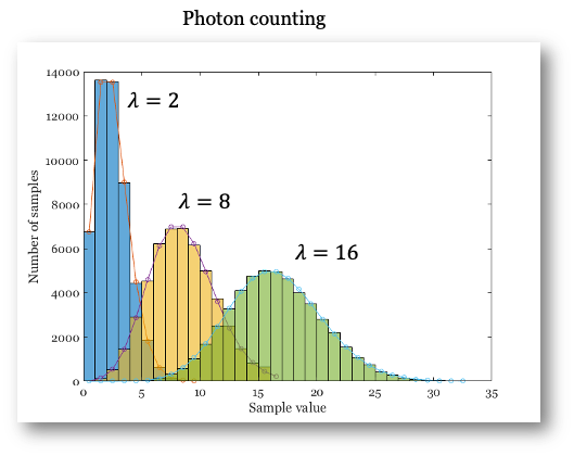
The Poisson formula describes the probability of observing \(n\) electron events, given a mean \(\lambda\): \[ P(n; \lambda) = \frac{\lambda^n e^{-\lambda}}{n!} \]
Here, \(\lambda\) is both the expected (mean) number of events and the variance of the distribution. For large \(\lambda\) (greater than about 15 or 20), the Poisson distribution closely resembles the Normal (Gaussian) distribution (Figure 14.5). The main differences are that the Poisson distribution only takes integer values and is skewed for small \(\lambda\). As \(\lambda\) increases, the distribution becomes more symmetric and approaches the Normal distribution.
A key fact we will use later: for a Poisson distribution, the mean and variance are equal. This property distinguishes Poisson noise from other types of noise.
You can see a step-by-step statistical explanation of photon arrivals followed by electron generation in the ISETCam script. The script demonstrates why, in conventional CMOS image sensors, both the incident photons and the resulting electrons follow Poisson statistics.
This relationship -Poisson distribution followed by another Poisson distribution- does not apply to other sensor types. When a photon absorption generates multiple electrons (photomultipliers and SPADs), the statistical distribution of the output requires some more thought (Section 20.10).
The history of these discoveries is fascinating but too detailed to cover here. For more, see these notes.↩︎