7 Geometric optics
The book is still taking shape, and your feedback is an important part of the process. Suggestions of all kinds are welcome—whether it’s fixing small errors, raising bigger questions, or offering new perspectives. I’ll do my best to respond, but please keep in mind that the text will continue to change significantly over the next two years.
You can share comments through GitHub Issues.
Feel free to open a new issue or join an existing discussion. To make feedback easier to address, please point to the section you have in mind—by section number or a short snippet of text. Adding a label characterizing your issue would also be helpful.
Last updated: November 6, 2025
7.1 Geometric optics overview
Modeling light as rays is a useful approximation for many calculations. This method enables us to use simple geometric calculations (e.g., similar triangles), to derive many properties of simple lenses. For this reason this approach is also called geometric optics. In this chapter we use geometric optics to describe the simplest image forming optics, a pinhole. After understanding the logic of modeling using rays and pinholes, I also explain the limitations of the ray model and why we will also model light as waves. Finally, I discuss the key concept of the point spread function, which plays a role in all the different modeling approaches. I extend the geometric optics calculations in the next few chapters, before turning to linear systems theory and wavefronts (Fourier optics).
7.2 Pinhole optics
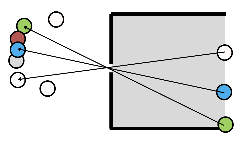
If we model light as a collection of rays, it is easy to understand why imaging through a pinhole produces an image (Figure 7.1). The figure shows a set of objects on the left. The camera is a dark chamber with only a pinhole opening. The image is formed on the planar surface, at the right. The light rays travel in a straight line, so only a small subset of the rays from each object passing through the pinhole. We can trace the light path by starting at a point on the image and drawing a straight line into the object space. The geometry illustrates how the rays from adjacent objects arrive at adjacent positions in the image plane, forming a reversed and inverted image.
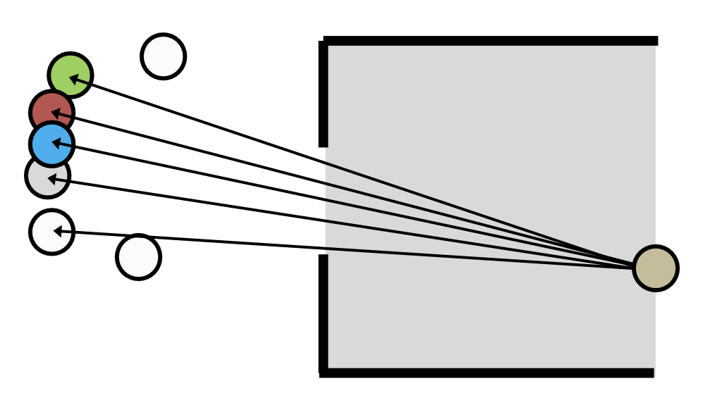
If the pinhole is small, each image point receives rays from a small region in object space (Figure 7.2). As we increase the pinhole diameter, each image point receives rays from larger regions on the objects. If multiple objects contribute rays to an image point, the image will be blurry. Conversely, according to the ray model, reducing the pinhole size should sharpen the image.
7.2.1 Parallel (collimated) rays
The rays from a point on an object often radiate in a wide range of directions. A special case -that is important in many practical applications- are the rays from distant points (Figure 7.3). When the point is far, only a small angular bundle of rays arrives at the pinhole. When the angle is very small, the rays are nearly parallel. In that case we say the beam of light is collimated.
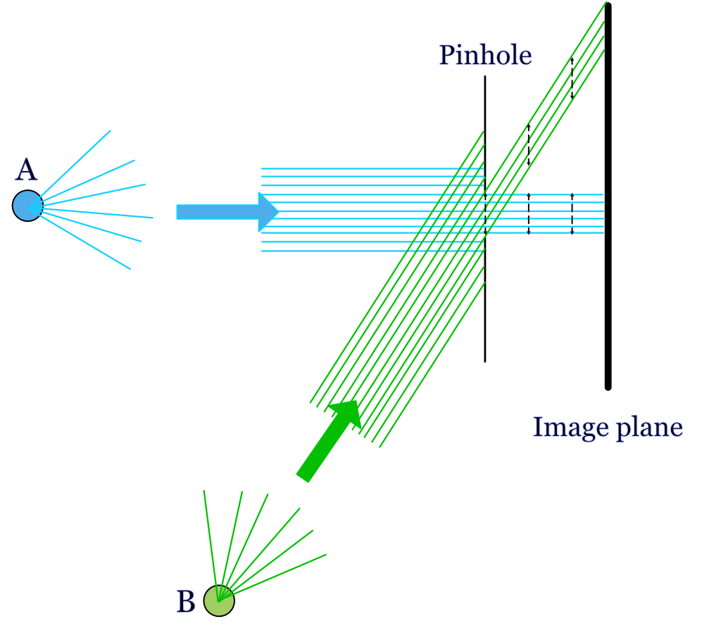
For an object point, A that is aligned with the pinhole (on-axis), the ray model of light predicts that the rays will continue straight through the pinhole aperture and form an image that is very close to the same size as the pinhole itself. Consider a distant off-axis point, B. Its rays, too, will start in many directions and only a narrow, collimated subset of rays will arrive at the pinhole aperture. Because of the angle between the collimated rays and the pinhole, a smaller fraction of the rays will pass through the pinhole aperture. There will be less light from B than from A. The relative amount of light that makes it through the pinhole depends on the cosine of the angle between the pinhole and the rays. But the shape of the image from the two points does not differ. If the pinhole is circular, on- and off-axis points will produce a circular image with the same diameter as the pinhole.
Figure 2.3 by Ayscough illustrates an image formed by a complex scene, with many points. Each point in the scene is blurred and rendered at a unique position. Also, the intensity at each point will be impacted by its relative angle to the pinhole and image surface. If the image intensity through the pinhole is adequate, and we do not mind the blurring, we will have a satisfactory image.
7.2.2 Pinhole: Computer graphics
Pinhole cameras are often used in computer graphics calculations. They are simple to compute, tracing light from the recording surface (film or sensor) through the pinhole back into object space. In computer graphics it is fairly common to aim to render a nice looking image, rather than a physically accurate image. The pinhole approximation to optics provides a sharp image with large depth of field that is suitable for many applications.
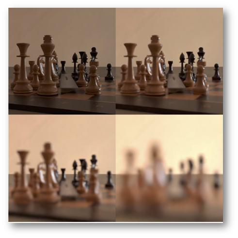
It is also possible to use pinhole computations to illustrate the limitations of this model in real image systems. In Figure 7.4 I rendered a chess set scene with the pieces, each a few cm tall, positioned about 0.5 meters from the pinhole camera. The four pictures were rendered using different pinhole diameters. The upper left allows only one ray through from each location in the scene. The aperture diameters for the next three pictures are for three different pinhole sizes. The images are brighter as the pinhole size increases. For this example, the image at the two smaller pinhole sizes are tolerable. Depending on your viewing distance from the screen or page, the third pinhole image might be usable. But the largest pinhole, which lets in the most light, loses so much spatial information that the individual pieces blur together in the image (Section 7.7).
7.2.3 Pinholes: real life
The basic idea of the pinhole camera (also called the camera obscura) has been known for thousands of years. Surely, many people noticed the phenomenon in different times and places. We have a record that the Chinese philosopher Mozi (c. 470–391 BC) wrote that an inverted image is formed through a pinhole, and moreover he explained the phenomenon by positing that light travels in straight lines! The Chinese scientist Shen Kuo (1031–1095) described the process explicitly in his book Dream Pool Essays, also noting that the image is inverted because light rays travel in a straight line from the source to the pinhole and then continue straight to form the image.
The most significant Islamic figure is Ibn al-Haytham (c. 965–1040), also known as Alhazen. His influential work, the Book of Optics, provides a comprehensive analysis of the camera obscura phenomenon. He used the term al-bayt al-muthlim (“the dark room”) to describe the pinhole camera, and he conducted experiments to demonstrate that a small hole could project an image of an external scene onto the opposite wall. Al-Haytham correctly reasoned that the pinhole created a clear image because it isolates and channels individual light rays from different points of the object, preventing them from mixing. His work included many other observations that laid the groundwork for modern optics.
From time-to-time people report on interesting examples of naturally occurring pinhole cameras. This video shows how the holes at the top of a curtain produce a series of overlaping images of the street below.
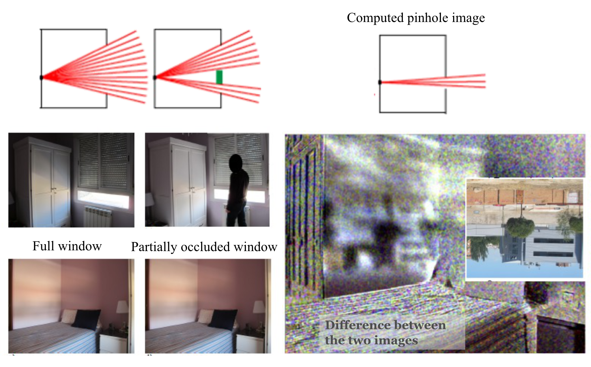
Torralba and Freeman (2012) described examples of naturally occurring pinhole cameras, and how to create a pinhole image computationally even when a window is too big to produce a useful image. They say you can take record the very blurry image from a large window opening, and then you can put a small occluder into the window (maybe stand sidewise in the middle of the window) and take a second image. Then, subtract the two images. By the Principle of Superposition, the difference image corresponds to the image when the aperture was the same size as the occluder. This method is more complex to implement because it involves acquiring two (linear) images and then subtracting them. And the world might have changed between the time you took the two image. But it’s a good trick for spies who are desperate to learn where they are being held hostage.
7.3 Diffraction
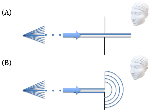
Useful as the ray model has been, for more than 300 years scientists have known that geometric optics is not completely accurate. Consider the simple prediction of the ray model in Figure 7.7. The parallel rays from a point source should pass through the pinhole and continue in a straight line, forming an image the size of the pinhole. An observer to the side should see only darkness, as no rays are heading toward their eyes.
But this isn’t what happens. As the Jesuit scientist Francesco Grimaldi, a contemporary of Newton, documented, light behaves in surprising ways near small apertures and edges (Grimaldi 1665). He observed that light spreads out, allowing the pinhole to be seen from the side and creating an image on a screen that can be larger than the pinhole itself. He gave the name diffraction to this phenomenon where light deviates from a straight path.
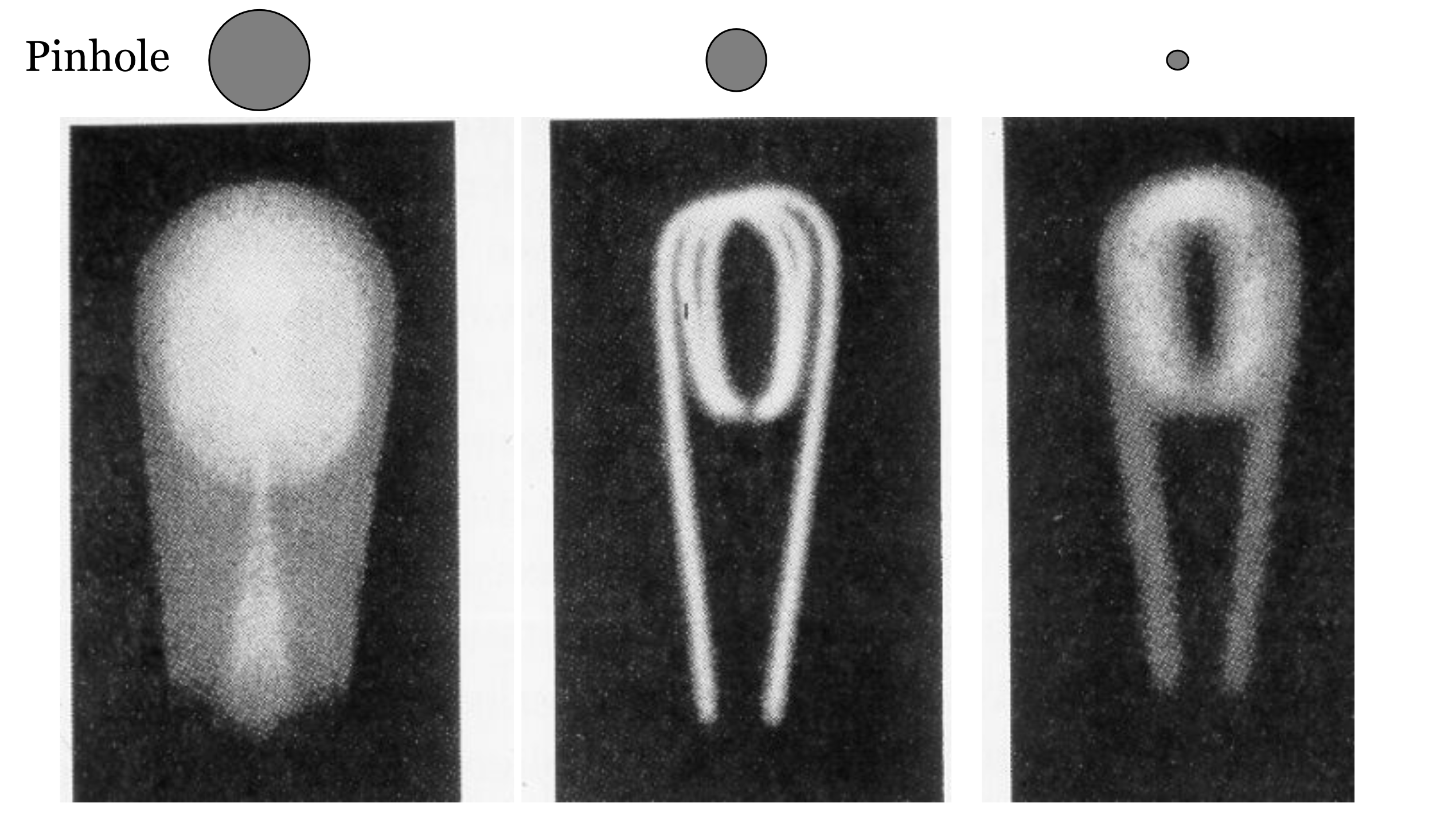
The trade-off between pinhole size and image sharpness provides a second, compelling example of diffraction. In their classic textbook, Jenkins and White showed a series of images of a light bulb filament through pinholes of decreasing size (Jenkins and White (1976)). As predicted by the ray model, reducing the pinhole size initially sharpens the image. But beyond a certain point, further reducing the pinhole size makes the image blurrier, directly contradicting the ray model. These observations demand an explanation that goes beyond geometric optics.
7.4 Huygens wave model
The Dutch scientist Christiaan Huygens, working at the same time as Newton, proposed an alternative to the ray model: he modeled light as waves expanding to fill space. In Huygens’ theory, light from a point source expands as a spherical wave. The leading edge of this expansion, the wavefront, can be seen as a collection of points, each acting as a source for a new secondary wavelet. This model successfully predicts many phenomena, including reflection from a mirror and the change in light’s direction (refraction) as it passes from one medium to another (Figure 7.9).
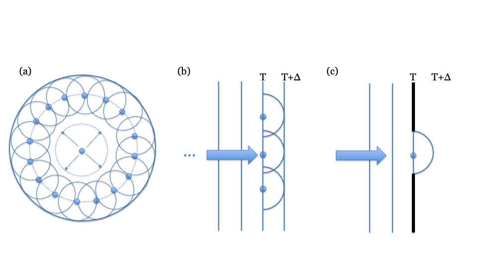
When a plane wave travels through open space, the constructive interference of all the secondary wavelets results in a new plane wave that propagates straight ahead, much like an ocean wave. However, when this wavefront passes through a small aperture or near an edge, the aperture blocks most of the secondary sources. The few wavelets that do pass through are revealed, causing the light to spread out spherically.
This directly explains diffraction. A very small pinhole allows only a tiny portion of the wavefront to pass, which then propagates outward as a nearly perfect spherical wave, allowing it to be seen from many directions. As the aperture size increases, more of the plane wave passes through, and the output more closely resembles a plane wave. This wave model elegantly explains why a pinhole’s effect on an image depends so critically on its size relative to the wavelength of light.
Although the ray and wave theories were proposed at about the same time, Newton’s 1704 framing of light as rays was widely accepted for roughly a century. Widespread recognition of the accuracy of Huygen’s wave theory was delayed until Thomas Young’s 1804 demonstration of the interference pattern created by light from two coherent, nearby sources. I find it interesting to learn about the the history of these ideas..
I have worked in fields where scientists rely mainly on hypothesis testing: they perform experiments to see if a theory is provably wrong. Surely Newton’s theory of light as a ray is provably wrong, and it was so proved more than 300 years ago! And yet, we use rays to describe light routinely. This is because in many cases the ray theory is an excellent approximation, and we use it as a simple way to reason about radiation - approximately.
This is a very pragmatic approach, which is deeply embedded in the mind of many scientists and engineers: Use the tool that is accurate enough for the problem at hand. Approach your problem with a toolbox of methods, and choose the one that gets the job done. In this spirit, the phrase ‘all models are wrong, some are useful’, Box (1976) is widely quoted in many engineering disciplines. In these fields hypotheses that are useful are included in the toolbox. It is essential to understand the scope over which the tool can be reasonably relied upon.
7.5 Double slit experiments
Grimaldi’s observations documenting how light spreads out after passing the edge of an obstacle or through a narrow slit, are easily reproducible and important. Huygens put forward a genuine wave theory of light. His principle of secondary wavelets elegantly explained reflection and refraction, and even hinted at diffraction (Huygens (1690)). It is surprising to me that Newton felt he could promote a ray theory of light despite these prior observations and theory. It was fascinating to learn that Newton and Huygens directly confronted one another on both optics and gravity (Shapiro (1989)). Perhaps because Newton was remarkable in so many ways, his voice dominated the scientific scene for decades.
Even though Huygens theory did account for many important phenomena; to me the simple observation in Figure 7.7 decisively demonstrates the necessity of a theory that allows for waves. Nonetheless, it wasn’t until Thomas Young presented his famous double-slit experiments to the Royal Society in 1801–1803 that Newton’s hold on the field began to loosen (Young (1804b)). This paper was a crucial step in the shift of the scientific consensus towards the wave theory of light. The ability to see the interference fringes provided quantitative, unmistakable proof of the value of the wave theory. Only waves, not particles, could add and cancel in this way and made the phenomenon hard to ignore. Young -and many others- considered- the demonstration of interference to be decisive1.
The experiment requires some precision, but it is fairly straightforward to instrument (Figure 7.10). One begins with a collimated beam arriving at a small aperture (part A). The light passing through the aperture serves as a coherent light source. It is allowed to transport forward to a second surface that has two narrow slits separated by some small distance. It is now the turn of these two slits to provide separated coherent light sources. When we observe the image formed by the double slits on a surface, the image is a striped pattern. As Young explained and drew in his original paper (part B), this is what one might expect of the two slits are both emitting waves at the same frequency.
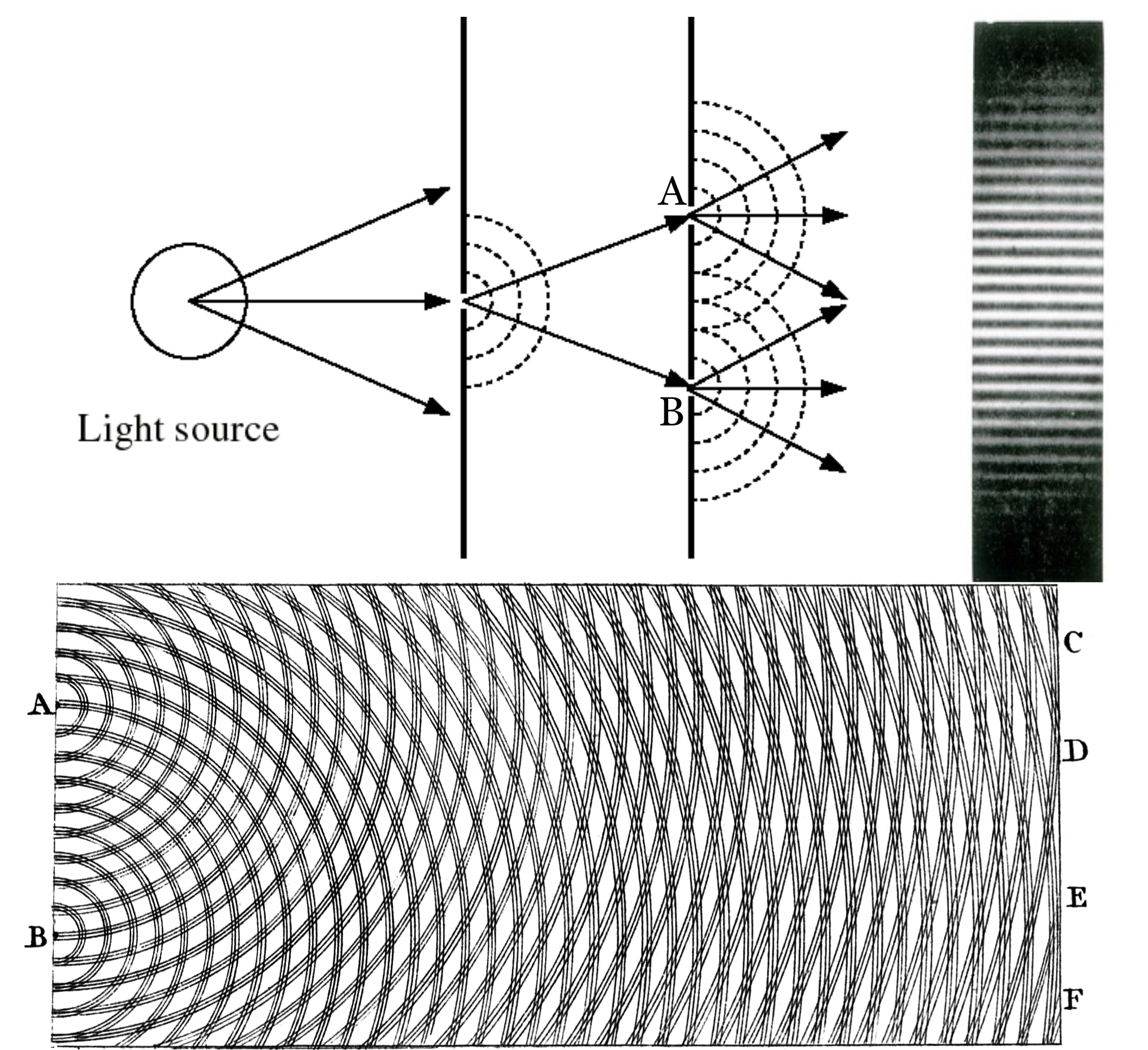
Even after Young’s presentations to the Royal Society, the wave theory met resistance. The loudest was from Henry Brougham who made personal attacks on Young2. But serious thinkers also wondered whether a wave theory could be right. What was the medium that supported the waves? Huygens referred to it, but the so-called ‘ether’ had not been measured3. And if the waves were propagating through a medium, wouldn’t inhomogeneities cause them to deviate from straight lines?
A particularly important event that turned the tide occurred a decade later, when Augustin-Jean Fresnel supplied the mathematics of diffraction and interference. This was a famous event in the history of physics. In 1818, Fresnel submitted his wave theory to a competition sponsored by the French Academy of Sciences. One of the judges, Siméon-Denis Poisson, was a staunch supporter of Newton’s particle theory and sought to disprove Fresnel’s work. Using Fresnel’s own equations, Poisson calculated that if a circular obstacle were illuminated by a point source of light, a bright spot should appear in the very center of the shadow. Poisson presented this as a reductio ad absurdum—an absurd conclusion that surely proved the wave theory was wrong.
However, the head of the committee, François Arago, decided to perform the experiment. To the astonishment of many, Arago observed the bright spot exactly as predicted. This dramatic confirmation of a counter-intuitive prediction was a decisive victory for the wave theory. The spot is now ironically known as Poisson’s spot (or sometimes Arago’s spot). This work ended the dominance of the corpuscular theory for some time. It was to return with Einstein’s work, which I explain in Chapter 14.
I was delighted to see the fundamental principle of the double-slit experiment return in my Inbox while writing this book. The core idea of the experiment is to measure the superposition of two signals. Even as technology has scaled, scientists continue to use this principle to investigate and characterize the properties of electromagnetic radiation.
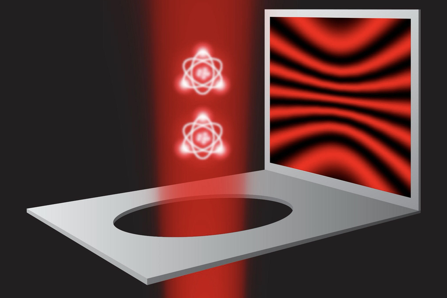
Here is a link to see the article in Physics World.
7.6 Polarization
(Maybe we introduce polarization here. Maybe earlier. Maybe put this in a callout instead of the moder double-slit callout.)
What kind of a wave is light?
Transverse or longitudinal wave. Polarization.
7.7 Pinhole size or diffraction: which blurs more?
From these simple considerations, we have seen that the image is blurred by two effects: the pinhole size and diffraction. Increasing the pinhole would create a larger spot on the wall, but decreasing the pinhole size reveals the spherical nature of the wavefront and also increases the size of the spot on the wall. We can compare the size of these two effects numerically.
First, consider what we expect from the ray model. If the pinhole diameter is \(D\), a far-away point on the main axis will produce a blurred spot in the image of size \(D\). Also, the pinhole-blur predicted by the ray model is the same no matter how far the image plane is from the pinhole.
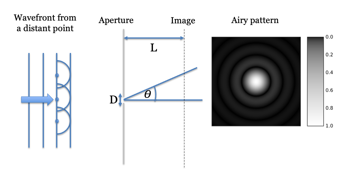
Second, consider the light pattern we expect for a plane wave passing through a pinhole aperture. This pattern can be calculated using a formula derived by the astronomer, George B. Airy (Airy 1835) and is shown in Figure 7.12. The Airy pattern has a central bright spot (the Airy disk), which is surrounded by a series of concentric rings. The size of the pattern depends on the wavelength of the light \(\lambda\), the diameter of the pinhole \(D\). Unlike the ray model, for the diffraction case the rays are expanding so that the distance \(L\) from the pinhole to the image plane matters. The image is radially symmetric with a bright spot in the center, surrounded by a set of concentric rings of decreasing intensity. The Airy disk contains about 85% of the total energy. The mathematical notation for the Airy pattern is a bit complex, but the diameter of the Airy disk, \(d\), has a simple formula
\[ d = 2.44~L~(\lambda / D) \tag{7.1}\]
Suppose we calculate the size of the diffraction diameter when the image plane is 1 m away, so \(L=1\), and for a wavelength of light is 550 nm. Suppose the pinhole diameter is \(D = 10^{-4} m\). The diameter of the Airy disk, \(d\), will be
\[ d = 2.44 \times (1 m) (550 \times 10^{-9} m )/ 1 \times 10^{-4}m) = 0.0134 m \tag{7.2}\]
The diffraction spread exceeds the pinhole spread when \(d\) exceeds \(D\). We do the calculation for different assumptions about the distance to the image plane ISETCam:fise_diffraction. As an example, we find that when the distance to the image plane is \(L = 1m\), the pinhole blur is larger than the diffraction blur for a pinhole diameter of about \(1 mm\). When the image plane distance, \(L\), is closer, say \(10 mm\), the pinhole blur exceeds the diffraction blur when the diameter is \(100 \mu\).
In a paper entitled “On the Diffraction of an Object-glass with Circular Aperture”, George Airy provided the mathematical description of the diffraction pattern (Airy 1835). A modern derivation of the full point spread function for both the circular aperture and other shapes is in Goodman (2022) (pages 88-94). The computation is implemented and frequently used in ISETCam. It is explained in this tutorial.
In the main text, we expressed the formula for a particular distance from the pinhole to an image plane. For a pinhole, the formula is usually given in terms of the angle of the bundle of rays emerging from the pinhole.
\[sin(\theta) = 1.22 \lambda / D\]
When the angle is small, \(\theta < 10 \deg\), the formula is very accurately approximated as
\[ \theta = 1.22 \lambda / D \]
The size of the spot on the image plane depends on the distance how far away the pinhole is from the pinhole, as you can see in Equation 9.5. In Chapter 9 we provide a formula for the Airy disk size for ideal lenses.
7.8 The point spread function
Throughout this section, we have analyzed optical systems by asking a simple question: what does the image of a single point of light look like? The resulting image pattern is called the point spread function (PSF), and it is a fundamental measure of optical performance. The Airy pattern, for example, is the PSF for a diffraction-limited circular aperture. We will encounter other types of PSFs when we analyze optical systems using linear systems theory (Chapter 11).
The PSF is a cornerstone of lens simulation, characterization, and computational imaging. Its importance stems from a crucial property of many optical systems: they are approximately linear. This means that the image of two points added together is the same as the sum of the images of each point individually (a property known as superposition).
Because of linearity, we can simulate the image of any complex scene. We can model the scene as a vast collection of individual light points. If we know the PSF, we can calculate the final image by scaling the PSF by the intensity of each point in the scene and summing all the resulting patterns. This process might involve millions of points, but it is a task that modern computers handle with ease.
In an idealized system, the PSF might be the same for every point in the scene, merely shifted in position. Such a system is called linear and space-invariant (LSI), and in that case the scaling and summing is called convolution. In most real-world optics, however, the system is space-variant: the PSF’s shape and size change depending on the point’s position in the field of view (e.g., its distance from the center, or field height).
The concept of building an image from the sum of PSFs is foundational, and we will use the ideas of linear systems throughout this book. The appendices provide more mathematical detail on general linear systems (Section 29.1) and the special case of LSI systems (Chapter 31).
7.9 Pinhole PSFs
7.9.1 Pinhole and distance
Even for a simple pinhole, the PSF isn’t a single, fixed pattern. Its shape depends on how far the light source is from the aperture. This distance determines which of two diffraction regimes applies.
When the point source is far away, its rays arrive collimated and thus the wavefront is a plane. This is the realm of Fraunhofer diffraction (or far-field diffraction). In this common scenario, the PSF for a circular pinhole is the classic Airy pattern we discussed earlier.
When the point source is close to the pinhole, its rays arrive diverging and the wavefront is a curved, spherical wavefront. This situation is described by Fresnel diffraction (or near-field diffraction). In the near field, the PSF’s shape and size change with the distance between the source and the pinhole.
7.9.2 Pinhole shapes
So far, we have focused on circular pinholes. This is a practical choice, as many apertures—from the human pupil to camera lenses—are approximately circular. A key advantage of a circular aperture is its rotational symmetry; rotating the camera (or your head) doesn’t change the image blur. The resulting PSF, like the Airy pattern, is also circularly symmetric and can be described simply by its radial profile.
However, both nature and technology provide many examples of non-circular apertures. These produce more complex, two-dimensional PSFs that are not rotationally symmetric. In the following sections, we will use an ISETCam script to explore how to calculate the diffraction-limited PSF for some of these interesting shapes.
7.9.2.1 Rectangular pinholes
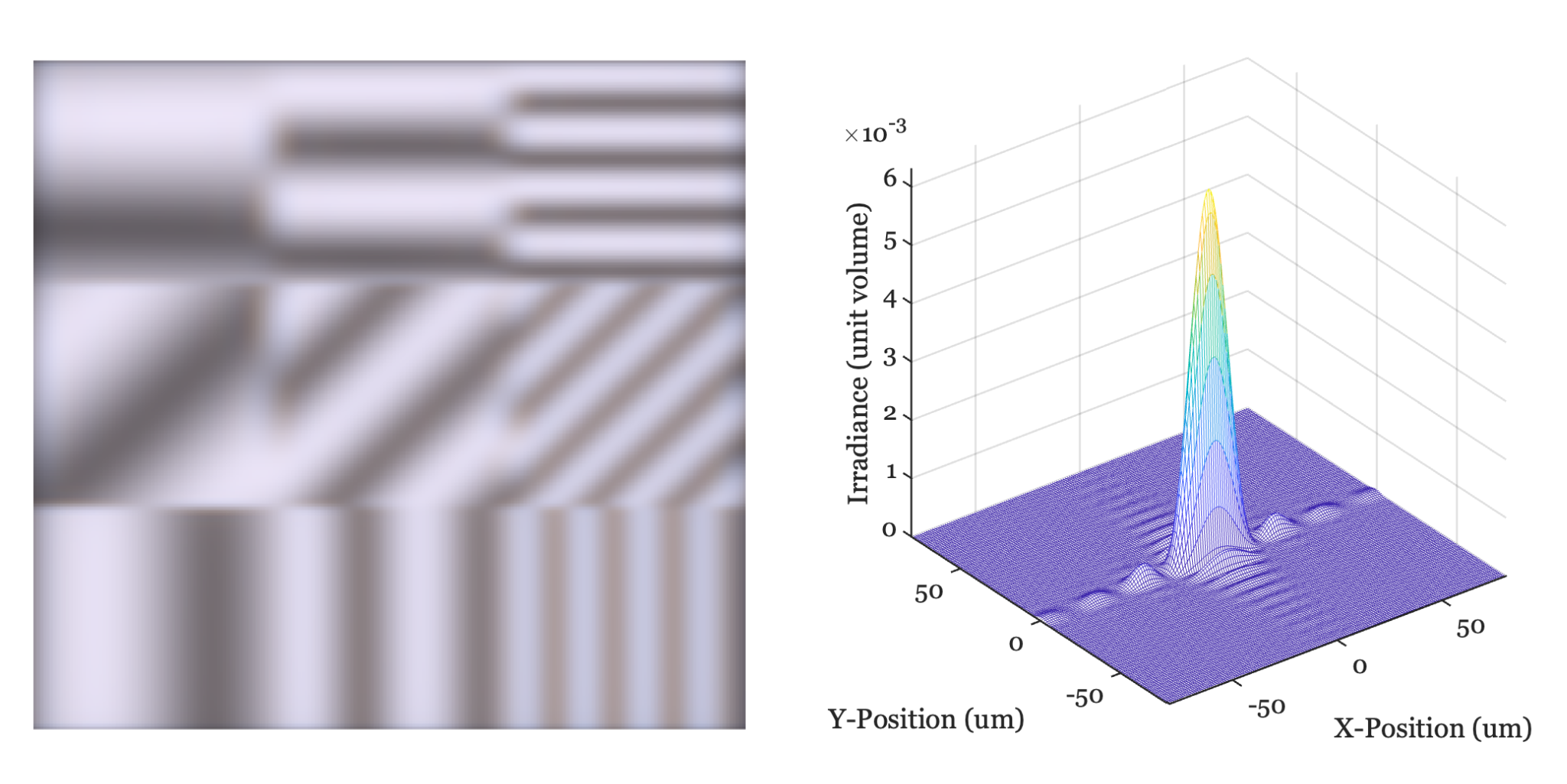
The script fise_oiAperture illustrates how to calculate the PSF for a rectangular aperture in ISETCam. An image computed using the PSF from a diffraction limited rectangular pinhole, and the PSF for that pinhole, are shown in Figure 7.13. The images illustrate a case for the rectangular aperture is three times wider (x) than high (y). The larger vertical height causes less blur in the y-direction, making the image sharper for the horizontal stripes.
There is a formula for the rectangular diffraction-limited PSF, given in terms of distance on the sensor surface.
\[ \text{PSF}(x',y') \;\propto\; \left[\operatorname{sinc}\!\left(\frac{\pi a}{\lambda f}\,x'\right)\right]^2 \;\left[\operatorname{sinc}\!\left(\frac{\pi b}{\lambda f}\,y'\right)\right]^2, \]
where \(a\) and \(b\) are the aperture widths in the \(x\) and \(y\) directions, \(f\) is the focal length, and \(\lambda\) is the wavelength. We define \(\operatorname{sinc}(u) = \tfrac{\sin(u)}{u}\).
In the script, you will see that I didn’t use the formula directly. Rather, I simply defined the shape of the aperture and ran a calculation. In Chapter 13 I will explain that calculation. Being able to numerically compute with the wavefront means we can find the PSF for many different shapes.
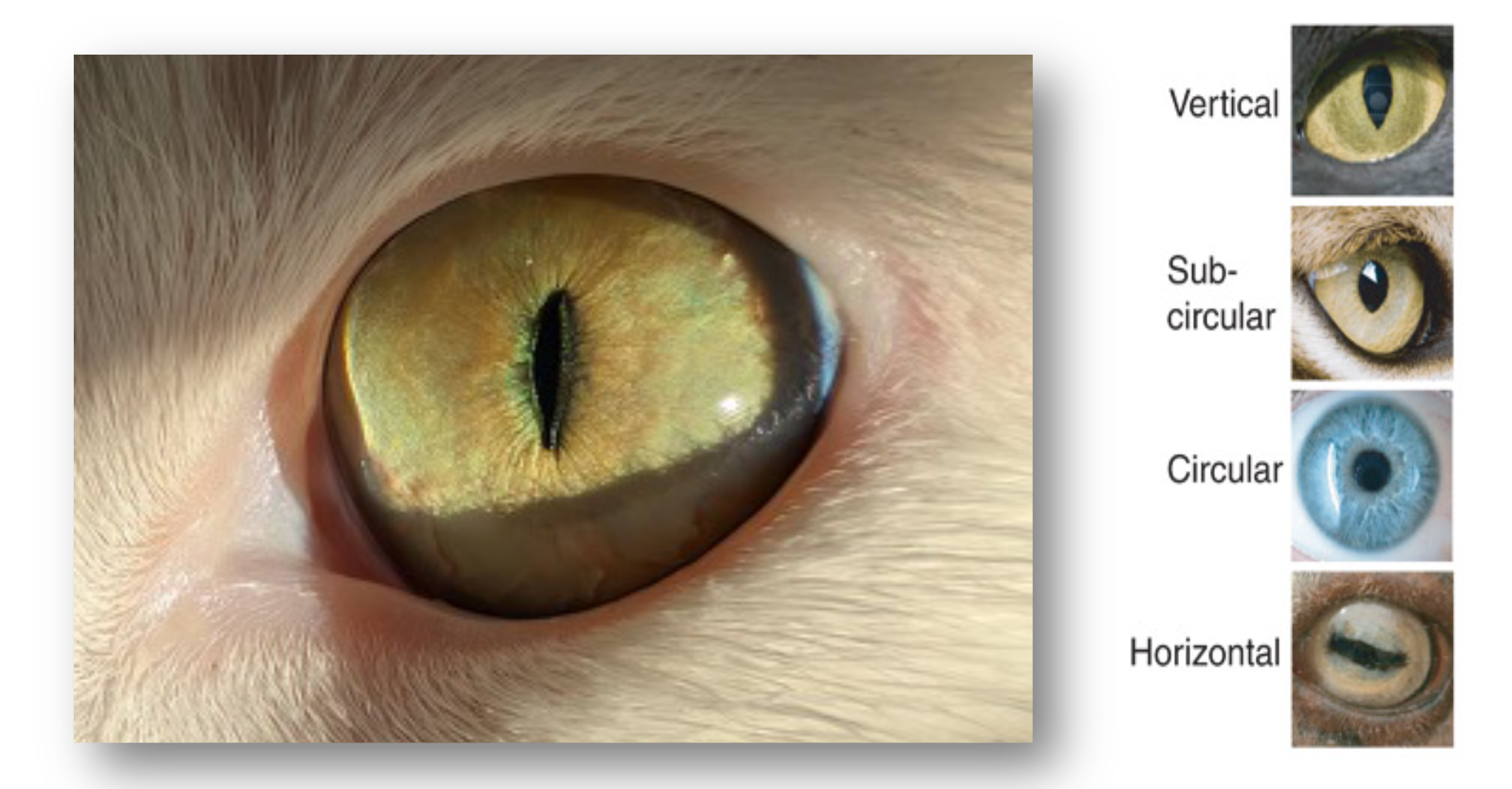
Approximately rectangular pupils are fairly common in biology, as well, and the pupil shape is associated with how they live their lives (Banks et al. (2015)). Vertically elongated pupils are associated with ambush predators that are active both day and night. So beware! Horizontally elongated pupils are more likely to be found in prey, who also have laterally placed eyes that helps them look all around.
7.9.2.2 Regular polygons
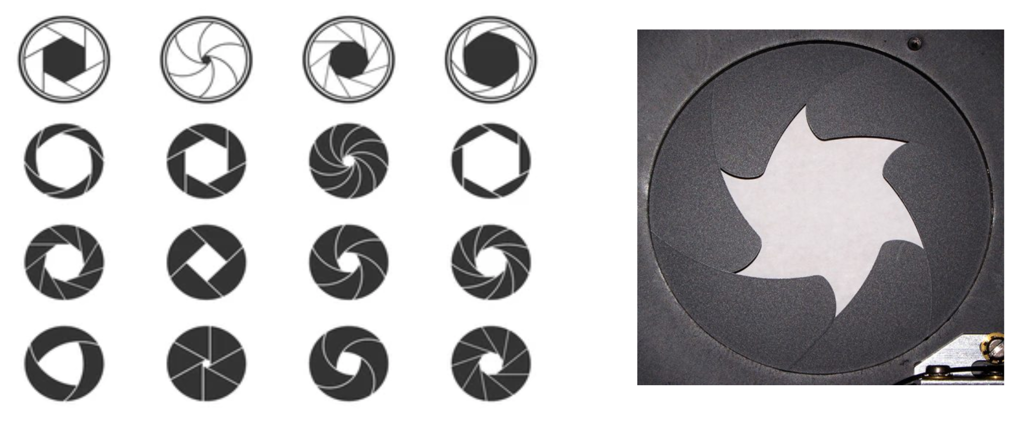
Classic cameras with mechanical shutters often had regular polygon shapes (left) or the interesting ‘leaf’ pattern at the right. These apertures introduce structure into the PSF that differs from a circularly symmetric aperture.
The impact of the regular polygon shape is quite visible in high dynamic range (HDR) scenes that include light sources. The script fise_oiAperture simulates an HDR scene, superimposing some very bright light sources on the background image. These apertures produce the flare pattern that one often sees in professional productions, including movies and sports shows. The three images show the flare pattern for polygons with different numbers of sides.
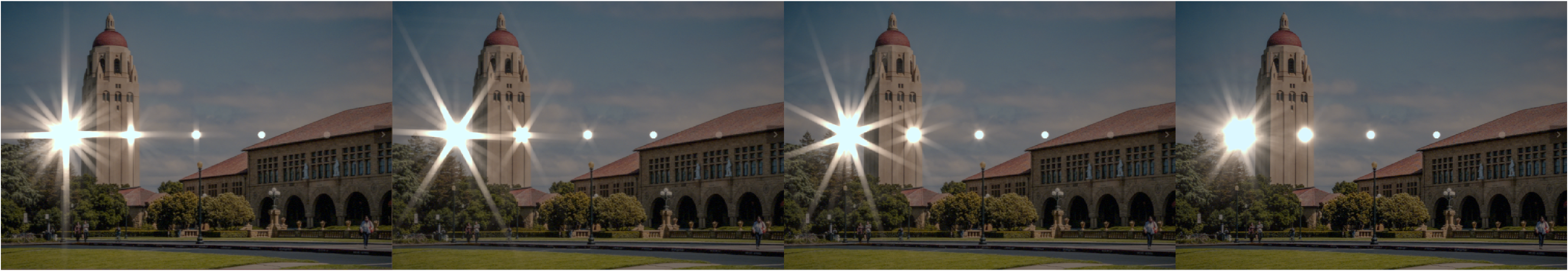
For the simulation in Figure 7.16, I also added some scratches and dust on to the lens for realism. The brightest light in each scene (left) is five orders of magnitude (\(10^5\)) more intense than the dimmest light (right), which is barely visible. The lights are all the same size, but the bright ones appear larger because of the blurring by the PSF.
7.9.3 Human PSF
Human eyes have approximately circular pupils. In bright light the pupil is contracted to about 3 mm diameter, and the PSF can be roughly circularly symmetric. In darker environments, the pupil widens and imperfections of the human optics (cornea, lens) often have a very large and irregular impact on the PSF. The pupil aperture is circular, but the optical imperfections distort the PSF and it takes on a very irregular shape (Thibos (2020) Thibos et al. (2002)).
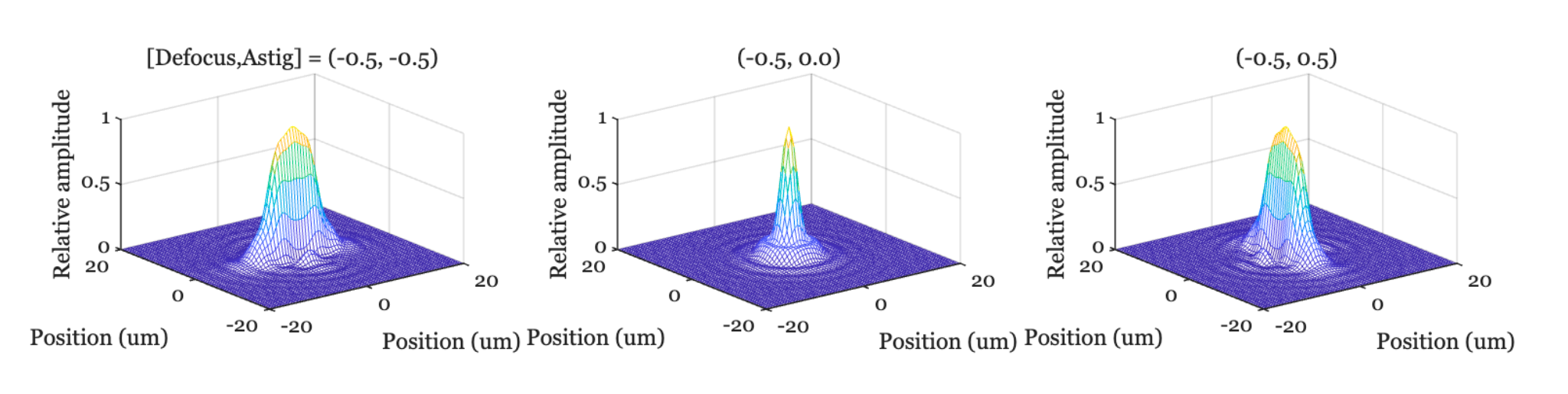
Even though the PSF is quite irregular, we often approximate its shape. One approximation summarizes whether or not the PSF is very different in two directions. If it is very different in two perpendicular directions, we say the person is astigmatic. Figure 7.17 shows PSFs with some defocus and astigmatism. These were simulated using the same wavefront methods I described above and that will be covered in Chapter 13.
I will show simulations of a range of human PSFs in Chapter 22. You can assess your own PSF easily. Glasses or contact lenses are typically designed to sharpen the PSF and counter any astigmatism. To see the PSF of your lens, take off your glasses or contact lenses, and look with one eye at a small spot of light in the dark -maybe a night light from across the room, or one of the LED lights on electronic gear- against in the presence of a uniform background such as a wall. The image you see is the PSF of your own visual system. If you are looking in a dark room, your pupil is probably relatively large. By squinting, you reduce the size of your eye’s aperture, and this is likely to sharpen the PSF. The squinting reduces how much the lens contributes to image formation. If the aperture is made quite small, say by using an artifical pupile, the image will be diffraction limited.
In making some experiments on the fringes of colours accompanying shadows, I have found so simple and so demonstrative a proof of the general law of the interference of two portions of light, which I have already endeavoured to establish, that I think it right to lay before the Royal Society, a short statement of the facts which appear to me so decisive (Young (1804b)).↩︎
Henry Brougham was a particularly fierce critique of Young’s entire research program and an ardent defender of Newton’s work. His strongest attacks were against Young’s important -and accurate!- observations about human color vision. More on that, including Young’s response (Young (1804a)) in Chapter 23.↩︎
“Now there is no doubt at all that light also comes from the luminous body to our eyes by some movement impressed on the matter which is between the two.”—Christiaan Huygens↩︎