6 Spatial regularities
The book is still taking shape, and your feedback is an important part of the process. Suggestions of all kinds are welcome—whether it’s fixing small errors, raising bigger questions, or offering new perspectives. I’ll do my best to respond, but please keep in mind that the text will continue to change significantly over the next two years.
You can share comments through GitHub Issues.
Feel free to open a new issue or join an existing discussion. To make feedback easier to address, please point to the section you have in mind—by section number or a short snippet of text. Adding a label characterizing your issue would also be helpful.
Last updated: October 4, 2025
6.1 Spatial regularities overview
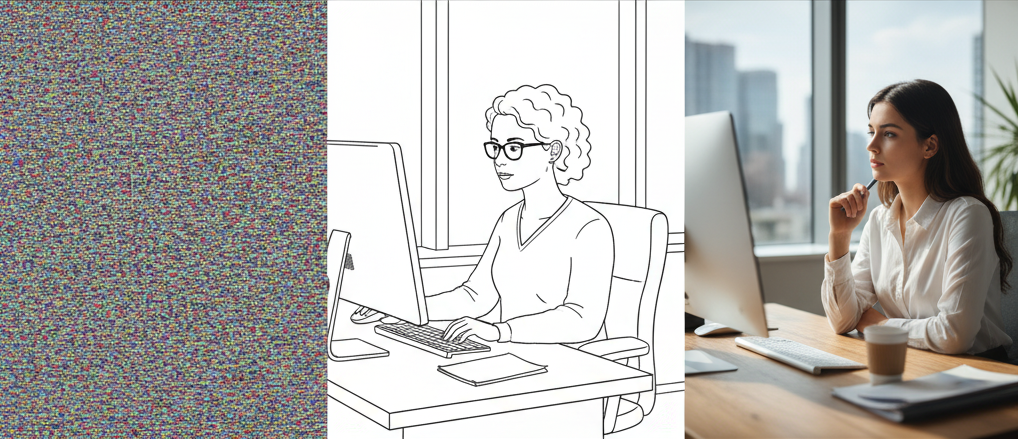
We can immediately recognize whether an image is natural or not. No reader will have any difficulty judging which of the three parts of the image is a natural image. Why? Plainly the natural image data conform to some spatial statistical rules that make them very distinguishable as a group.
We have already seen how information about the spectral characteristics of natural images can be helpful in interpreting them. Learning more about the spatial statistics of natural images -or not- has been a longstanding goal of image systems engineering and vision science. The reason is simple: the more we know about these statistics, the better we can do at interpreting the images we measure. For example, we should be able to remove noise more effectively by rewriting a noisy capture in a format that is more natural-like. We can even hope that we should be able to develop better algorithms to interpret the contents of the images (Section 4.2).
Over the last four decades, our knowledge about the spatial statistics has grown considerably. The development of machine learning algorithms, particularly diffusion methods for generating natural images, has been a recent striking advance. In this chapter we will start with the foundations and work our way towards the most recent insights.
6.2 Spatial correlations
Image scientists were immediately drawn to analyzing the very different spatial statistics of images. If we examine the three sections of Figure 6.1, one very obvious feature jumps out. In the first panel, every pixel is completely independent of the other. In natural images, if you know the light at one point there is a good chance that it will be similar to the light at another point. There are various mathematical ways to express this basic insight. And of course these measures all can be connected to one another, although sometimes with some difficulty.
6.3 Natural scenes and the 1/f spatial frequency falloff
Who first pointed this out? Relationship to the scale invariant idea of fractals, and the fractal nature of many things.
Ruderman and Bialek paper on natural image statistics.
Field, Olshausen
The scale invariance of natural images arises from their power-law spectral decay, which mathematically ensures statistical consistency across spatial scales. The connection between \(\fract{1}{f}^\alpha\) spectra and scale invariance can be expressed through:
The power spectrum of natural images follows:
\[ P(\omega) \propto \frac{1}{|\omega|^{2-\eta}} \quad \text{where } \eta \approx 0.8\text{--}1.5 \]
Here, \(\omega\) represents spatial frequency magnitude, and \(\eta\) controls the decay rate1,2,3.
For scale invariance under spatial scaling \(x \to \lambda x\), the power spectrum must satisfy:
\[ P(\lambda\omega) = \lambda^{-\kappa}P(\omega) \]
Substituting the power-law form:
\[ P(\lambda\omega) = \frac{1}{|\lambda\omega|^{2-\eta}} = \lambda^{-(2-\eta)}P(\omega) \]
This matches the scale-invariance condition with \(\kappa = 2-\eta\), demonstrating that statistical properties remain consistent across scales4,5,6.
6.4 The dead leaves model
Lee et al. (2001)
Jon’s Matlab script as a basis for discussing this. Software from Jon showing 1/f issues.
Also, the deadleaves function in ISETCam.
6.4.1 Scale invariance
Fractal connection The power-law exponent relates to fractal dimension \(D\) through:
\[ D = 3 - \frac{\eta}{2} \]
where \(D\) quantifies space-filling characteristics. Natural images typically exhibit \(D \approx 2.2\text{--}2.6\), consistent with their 1/f^α spectra7,8.
This mathematical framework shows that 1/f^α spectra inherently encode fractal, scale-invariant structure - the same statistical regularities appear whether analyzing fine details or coarse features of natural scenes9,10,11.
6.5 Diffusion models
Diffusion neural networks.
Eero’s analysis of the statistical properties of images using diffusion models.
6.6 Applications
Image compression and JPEG is the big one. It doesn’t get us all the way to objects. But it sure mattered.
https://people.csail.mit.edu/danielzoran/zoranweiss09.pdf↩︎
https://web.mit.edu/torralba/www/ne3302.pdf↩︎
https://www.sciencedirect.com/science/article/pii/0042698996000028↩︎
https://people.csail.mit.edu/danielzoran/zoranweiss09.pdf↩︎
https://web.mit.edu/torralba/www/ne3302.pdf↩︎
http://vigir.missouri.edu/~gdesouza/Research/Conference_CDs/IEEE_ICCV_2009/contents/pdf/iccv2009_285.pdf↩︎
https://people.csail.mit.edu/danielzoran/zoranweiss09.pdf↩︎
https://www.nature.com/articles/srep46672↩︎
https://people.csail.mit.edu/danielzoran/zoranweiss09.pdf↩︎
https://web.mit.edu/torralba/www/ne3302.pdf↩︎
http://vigir.missouri.edu/~gdesouza/Research/Conference_CDs/IEEE_ICCV_2009/contents/pdf/iccv2009_285.pdf –>↩︎