27 Spatial pattern sensitivity and metrics
Suggestions of all kinds for this book draft are welcome — whether it’s fixing small errors, raising bigger questions, or offering new perspectives. Please share comments through GitHub Issues. To make feedback easier to address, please point to the section you have in mind — by section number or a short snippet of text.
27.1 Spatial metrics overview
How can we evaluate the design of a camera? Lord Kelvin put it in that lovely style of the British upper crust
when you can measure what you are speaking about, and express it in numbers, you know something about it; but when you cannot measure it, when you cannot express it in numbers, your knowledge is of a meagre and unsatisfactory kind (Popular Lectures and Addresses “Electrical Units of Measurement” (1889).)
Goodhart’s Law as a warning: “When a measure becomes a target, it ceases to be a good measure.”
The answer depends on your intended use. If the camera is intended to create images that people see, then the design must be guided by the capabilities and limits of the human eye. If the camera serves as input to a robot, or a self-driving car, or a medical image diagnostic system, we expect the camera’s design to be evaluated by how well it assists those systems.
Engineering progress relies on measurement. Improving a system is an iterative process that involves a loop of designing, measuring, and redesigning. Consequently, performance metrics are fundamental to nearly all engineering disciplines.
It is also a common principle that systems of even moderate complexity have more than one performance measure. We are often forced to make trade-offs, for example, between a system’s speed and its accuracy. We see this in modern AI systems that offer a choice between a ‘fast’ mode and a more thorough ‘thinking’ mode.
Imaging systems are no different. They present numerous trade-offs. For instance, increasing a sensor’s spatial resolution can reduce the number of photons captured per pixel, thus lowering the signal-to-noise ratio (SNR). Conversely, increasing SNR by using wider color filter bandwidths may reduce color accuracy.
When there is only one parameter to optimize, assessing system design is straightforward. However, most systems involve optimizing multiple parameters simultaneously. A design change might improve some metrics while degrading others, making it difficult to determine an overall improvement.
This complexity is reflected in the field of image quality metrics. Many different metrics exist. Some assess a specific aspect of system performance, guiding the design of a particular component. Others, however, aim to capture the general notion of image quality as a human would judge it. The most famous of these—the Structural Similarity Index Measure (SSIM), with over 100,000 citations—is a prime example.
Engineers, computer scientists, and product managers often desire a single number they can optimize and market. As a student or young researcher, you might be tempted to resist this simplification. A word of advice: understand the limitations of single-number metrics, but don’t let their imperfection stall your progress. Use them as the valuable, albeit incomplete, tools they are.
In the image processing section, I introduce a number of image systems metrics that are designed to evaluate the system and its components directly (Section 36.1). Those metrics might assess the signal-to-noise (SNR) of a pixel, or the MTF of a lens.
In this chapter and in Chapter 29, I review metrics that are designed with the human viewer in mind: How sharp will the image appear? Will the noise be visible? Do the colors in the rendering match those in the original? This chapter covers spatial pattern sensitivity and metrics that depend on spatial (and temporal) image properties, such as sharpness, contrast sensitivity, and noise visibility. After we develop the principles of human wavelength encoding (Chapter 28), Chapter 29 covers color representations, CIELAB, and Spatial-CIELAB (S-CIELAB).
27.2 Spatial sensitivity in the transform domain
The usefulness of the analyses in the transform domain, in engineering generally and optics specifically, led vision scientists to ask whether measurements using harmonics could be useful for understanding and characterizing the human visual system. Perhaps the first person to see the potential application was the image systems engineer Otto Schade. This is the person who developed the concept of the modulation transfer function (MTF) for image systems engineering questions (Section 14.4.2).
I created four Google docs with historical information about CSF measurements, how to download the historical data, and how to imlement the modern models of the historical and more modern data. Integrate those pages here and write some Matlab scripts to create figures.
Show the data he collected of the CSF (1/MTF) he measured that I include in FOV. Maybe in the human spatial encoding chapter.
The use of harmonics to probe the visual system is quite different from their use in studying typical systems. At many points in this volume I have pointed out that harmonics are particularly valuable stimuli for space-invariant linear systems Chapter 39. These systems have an input and an output. THe use of harmonic stimuli in human vision faces two significant limitations. First, as we have just seen, the system is not at all space-invariant (Figure 26.7). It is justifiable to use harmonics as special stimuli over small regions of the retina, which can be close to space-invariant. Stimuli that span more than a degree or two will not have the special property (harmonics being nearly eigenfunctions) that make them so useful in systems analysis.
Second, even at the earliest stages of vision the neural encoding is not restricted to a single system.
27.2.1 Contrast sensitivity functions (CSF)
Optical scientists use both the space domain (PSF) and the transform domain (MTF) to study their system, and vision scientists use both domains as well. The nonuniformity of the optical blur, coupled with the nonuniformity of the cone spatial sampling, imply that shift-invariant methods only make sense over patches of the visual field. As a result, the carefully controlled harmonics used in vision experiments are modulated over relatively small regions of space.
There are several ways in which this modulation is accomplished in experiments, though perhaps the most common is to use a Gabor function; named after Denis Gabor, the Nobel Laureate credited with the discovery of the laser.
\[ \begin{aligned} g(x,y) &= \exp\!\left( -\frac{(x - x_0)^2 + (y - y_0)^2}{2\sigma^2} \right) [1 + a \cos\!\big(2\pi f x + \phi\big)] \end{aligned} \tag{27.1}\]
Gabor functions are harmonics modulated by a Gaussian. The standard deviation of the Gaussian (\(\sigma\)) controls the spatial spread; the frequency of the harmonic \(f\), controls the center frequency of the image. The phase term, \(\phi\), controls the spatial relationship between the harmonic and the peak of the Gaussian. The central position in the visual field is \((x_0,y_0)\), and the amplitude of the harmonic is controlled by \(a\).
Figure: Show images of different Gabors.
Show classic contrast sensitivity functions (CSF) measured with Gabor patches shown here.
Note: Should we adjust \(f\) and \(\sigma\) together, or should we fix \(\sigma\) and adjust \(f\) on its own. Thinking about the space-variant part of the human visual system, we realize both are important parameters.
27.2.2 Vernier acuity
Gerald and Suzanne lead the discussion of Vernier acuity.
https://www.fisicanet.com.ar/biografias/cientificos/v/vernier-pierre.php
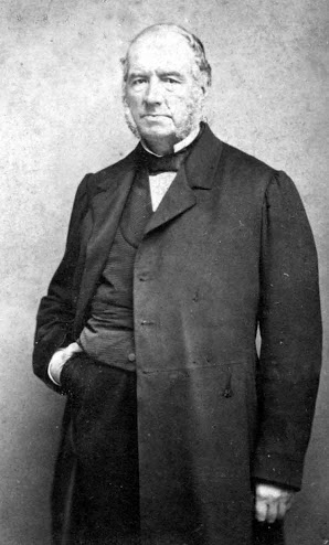
Something about Vernier calipers and the story of Pierre Vernier.
Historical
https://en.wikisource.org/wiki/1911_Encyclop%C3%A6dia_Britannica/Vernier,_Pierre
27.3 Spatial image quality metrics
I have links to both original measurements, modern measurements (Standard Spatial Observer), and many commercial versions of spatial metrics that are implemented in ISETCam. This section will describe those.
27.3.1 Classical single-channel metrics
That single channel guy with his metric and formula. Repeated everywhere. Barten. SQRI.
Earlier single channel. Value of multiple channel metrics? Existence?
27.3.2 Modern structural and perceptual metrics
SSIM and MS-SSIM
LPIP goes here because it is human judgments of image quality?
Pyramid from Beau? Multi-parameter
I forked the Mantiuk github repository: The Mantiuk repository is here:. His metric goes here, I think. His code reads classic datasets. Maybe we include the data files in the book?
The surprising metric LPIPS
27.4 Temporal sensitivity and metrics
Temporal MTF metrics, flicker visibility, and motion blur.